传统ARIMA步骤：

加载数据：模型建立的第一步当然是加载数据集。

预处理：取决于数据集，预处理的步骤将被定义。这将包括创建时间戳、转换日期/时间列的dType、制作系列单变量等。

使系列平稳：为了满足假设，有必要使系列平稳。这将包括检查序列的平稳性和执行所需的变换。

确定值：为了使序列平稳，将执行差值操作的次数作为d值

创建ACF和PACF图：这是ARIMA实施中最重要的一步。ACF PACF图用于确定我们的ARIMA模型的输入参数。

确定p和q值：从前一步的图中读取p和q的值

拟合ARIMA模型：使用处理后的数据和我们先前步骤计算的参数值，拟合ARIMA模型

预测集上的预测值：预测未来价值

计算MSE或者RMSE：为了检查模型的性能，使用验证集上的预测和实际值检查MSE或者RMSE值

在实现的过程使用SARIMAX实现，这是一个包含季节趋势因素的ARIMA模型。

下面直接上代码：

data：直接采用  facebook 的prophet时序算法中examples的数据，可以在git上下载。

begin：

# Load data
df = pd.read_csv('data/example_air_passengers.csv')
df.ds = pd.to_datetime(df.ds)
df.index = df.ds
df.drop(['ds'], axis=1, inplace=True)

              y
ds             
1949-01-01  112
1949-02-01  118
1949-03-01  132
1949-04-01  129
1949-05-01  121

# Resampling
df_month = df.resample('M').mean()
print(df_month.head())
              y
ds             
1949-01-31  112
1949-02-28  118
1949-03-31  132
1949-04-30  129
1949-05-31  121

# 拆分预测集及验证集
df_month_test = df_month[-5:]
print(df_month_test.tail())
print('df_month_test', len(df_month_test))
df_month = df_month[:-5]
print('df_month', len(df_month))

# PLOTS
fig = plt.figure(figsize=[15, 7])
plt.suptitle('sales, mean', fontsize=22)

plt.plot(df_month.y, '-', label='By Months')
plt.legend()

# plt.tight_layout()
plt.show()

# 看趋势
plt.figure(figsize=[15, 7])
sm.tsa.seasonal_decompose(df_month.y).plot()
print("air_passengers test: p={}".format( adfuller(df_month.y)[1]))
# air_passengers test: p=0.996129346920727

# Box-Cox Transformations ts序列转换
df_month['y_box'], lmbda = stats.boxcox(df_month.y)
print("air_passengers test: p={}".format(adfuller(df_month.y_box)[1]))
# air_passengers test: p=0.7011194980409873

下一步观察季节差分及趋势差分，找出m及d。

# Seasonal differentiation
# 季节性差分确定sax中m参数
df_month['y_box_diff'] = df_month['y_box'] - df_month['y_box'].shift(12)

# 做个例子 
最后得到的pvalue test diff13: p=0.000418 证明序列是稳定的。

下面进行模型选择及预测输出指标：

# SARIMAX参数说明
 '''
    趋势参数：（与ARIMA模型相同）
    p：趋势自回归阶数。
    d：趋势差分阶数。
    q：趋势移动平均阶数。
    
    季节性参数：
    P：季节性自回归阶数。
    D：季节性差分阶数。
    Q：季节性移动平均阶数。
    m：单个季节期间的时间步数。
 '''

# Initial approximation of parameters
    Qs = range(0, 3)
    qs = range(0, 3)
    Ps = range(0, 3)
    ps = range(0, 3)
    D = 1
    d = 1

    parameters = product(ps, qs, Ps, Qs)
    parameters_list = list(parameters)
    # list参数列表
    print('parameters_list:{}'.format(parameters_list))
    print(len(parameters_list))

    results = []
    best_aic = float("inf")

    for parameters in parameters_list:
        try:
            # SARIMAX 训练的时候用到转换之后的ts
            model = sm.tsa.statespace.SARIMAX(df_month.y_box, order=(parameters[0], d, parameters[1]),
                                              seasonal_order=(parameters[2], D, parameters[3], 12)).fit(disp=-1)
        except ValueError:
            print('wrong parameters:', parameters)
            continue

        aic = model.aic
        if aic < best_aic:
            best_model = model
            best_aic = aic
            best_param = parameters
        results.append([parameters, model.aic])

    result_table = pd.DataFrame(results)
    result_table.columns = ['parameters', 'aic']
    print(result_table.sort_values(by='aic', ascending=True).head())
    print(best_model.summary())
# Model:             SARIMAX(0, 1, 1)x(1, 1, 2, 12) 

得到 best_model 同时可以观察acf(resid)

sm.graphics.tsa.plot_acf(best_model.resid[13:].values.squeeze(), lags=48, ax=ax)

# 下图是对残差进行的检验。可以确认服从正太分布，且不存在滞后效应。
best_model.plot_diagnostics(lags=30, figsize=(16, 12))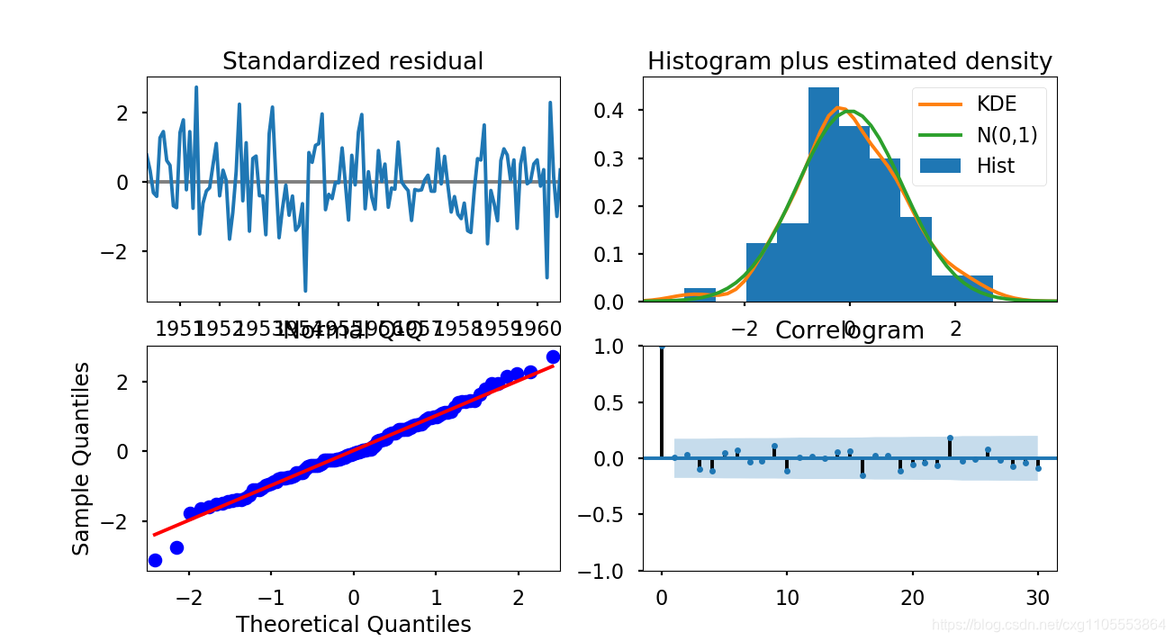

验证结束之后最后对测试集预测并输出指标mse及rmse

df_month2 = df_month_test[['y']]
# best_model.predict()  设定开始结束时间
# invboxcox函数用于还愿boxcox序列
df_month2['forecast'] = invboxcox(best_model.forecast(steps=5), lmbda)
plt.figure(figsize=(15,7))
df_month2.y.plot()
df_month2.forecast.plot(color='r', ls='--', label='Predicted Sales')
plt.show()

# 获取mse
print('mean_squared_error: {}'.format(mean_squared_error(df_month2.y,  df_month2.forecast)))

最后结果：#mean_squared_error: 90.93184037574731

结尾：

TS模块后续陆续更新auto_arima及lstm相应的概述及代码实现。