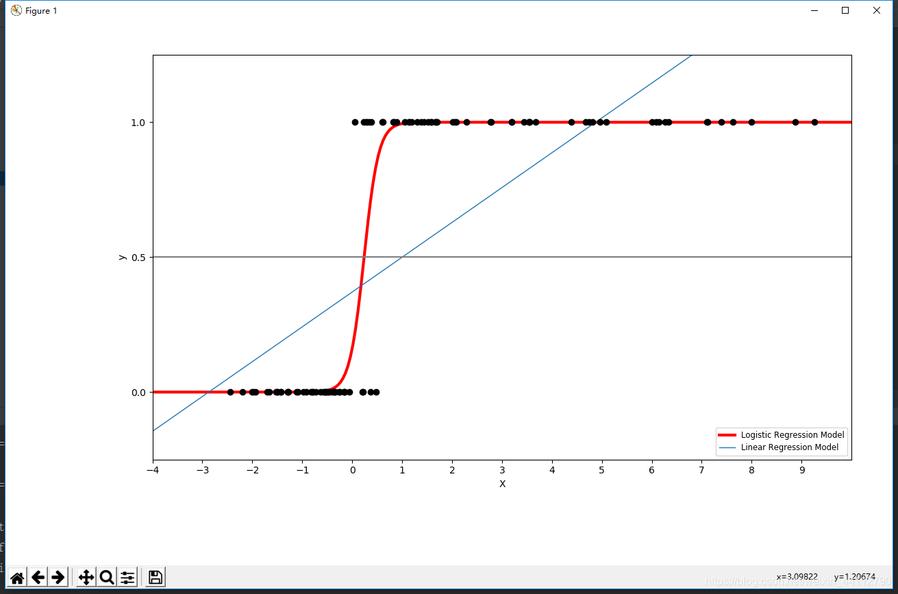
二分类

import numpy as np
import matplotlib.pyplot as plt

from sklearn import linear_model
from scipy.special import expit

# General a toy dataset:s it's just a straight line with some Gaussian noise:
xmin, xmax = -5, 5
n_samples = 100
np.random.seed(0)
# 构造协变量
X = np.random.normal(size=n_samples)
# 构造相应变量：将布尔值转为0-1
y = (X > 0).astype(np.float)
# 放大X > 0的部分数据，使得数据非对称
X[X > 0] *= 4
# 增加数据的扰动
X += .3 * np.random.normal(size=n_samples)
# 增加一列None，这里类似于转置但不能用X.T
X = X[:, np.newaxis]
# 构造逻辑回归分类对象
clf = linear_model.LogisticRegression(C=1e5, solver='lbfgs')
# 逻辑回归进行训练
clf.fit(X, y)
# and plot the result
plt.figure(1, figsize=(4, 3))
# 清空画布
plt.clf()
# 绘制训练集的散点图
plt.scatter(X.ravel(), y, color='black', zorder=20)
# 生成测试数据
X_test = np.linspace(-5, 10, 300)
# 预测测试数据
loss = expit(X_test * clf.coef_ + clf.intercept_).ravel()
# 绘制逻辑回归的曲线
plt.plot(X_test, loss, color='red', linewidth=3)
# 构造最小二乘对象
ols = linear_model.LinearRegression()
# 最小二乘法求解
ols.fit(X, y)
# 最小二乘法预测并绘制直线
plt.plot(X_test, ols.coef_ * X_test + ols.intercept_, linewidth=1)
# 绘制中线
plt.axhline(.5, color='.5')
# 标注绘图信息
plt.ylabel('y')
plt.xlabel('X')
plt.xticks(range(-5, 10))
plt.yticks([0, 0.5, 1])
plt.ylim(-.25, 1.25)
plt.xlim(-4, 10)
plt.legend(('Logistic Regression Model', 'Linear Regression Model'),
           loc="lower right", fontsize='small')
plt.tight_layout()
plt.show()
1
2
3
4
5
6
7
8
9
10
11
12
13
14
15
16
17
18
19
20
21
22
23
24
25
26
27
28
29
30
31
32
33
34
35
36
37
38
39
40
41
42
43
44
45
46
47
48
49
50
51
52
53
54
55

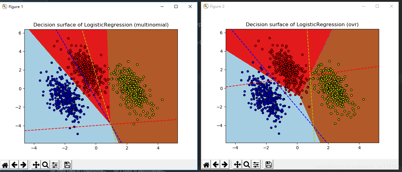
多分类

import numpy as np
import matplotlib.pyplot as plt
from sklearn.datasets import make_blobs
from sklearn.linear_model import LogisticRegression

# make 3-class dataset for classification
centers = [[-5, 0], [0, 1.5], [5, -1]]      # 样本中心
# 根据三个中心生成1000个样本，随机数种子为40
X, y = make_blobs(n_samples=1000, centers=centers, random_state=40)
transformation = [[0.4, 0.2], [-0.4, 1.2]]
# 通过内积干扰原来的数据
X = np.dot(X, transformation)

# 分别计算ovo与ovr方法
for multi_class in ('multinomial', 'ovr'):
    # 构造逻辑回归对象并训练
    clf = LogisticRegression(solver='sag', max_iter=100, random_state=42,
                             multi_class=multi_class).fit(X, y)

    # print the training scores
    print("training score : %.3f (%s)" % (clf.score(X, y), multi_class))

    # create a mesh to plot in
    h = .02  # 网格点矩阵的步长
    x_min, x_max = X[:, 0].min() - 1, X[:, 0].max() + 1     # x的边界
    y_min, y_max = X[:, 1].min() - 1, X[:, 1].max() + 1     # y的边界
    xx, yy = np.meshgrid(np.arange(x_min, x_max, h),        # 生成网格点测试数据
                         np.arange(y_min, y_max, h))

    # Plot the decision boundary. For that, we will assign a color to each
    # point in the mesh [x_min, x_max]x[y_min, y_max].
    Z = clf.predict(np.c_[xx.ravel(), yy.ravel()])      # 扁平化数据
    # Put the result into a color plot
    Z = Z.reshape(xx.shape) # 预测结果形状还原到扁平化之前

    plt.figure()    # 新的绘图窗口
    plt.contourf(xx, yy, Z, cmap=plt.cm.Paired)         # 绘制决策边界并填充颜色
    plt.title("Decision surface of LogisticRegression (%s)" % multi_class)  # 标题
    plt.axis('tight')    # 坐标轴适应数据量

    # Plot also the training points
    colors = "bry"
     # 绘制预测结果
    for i, color in zip(clf.classes_, colors):
        idx = np.where(y == i)
        # 散点图
        plt.scatter(X[idx, 0], X[idx, 1], c=color, cmap=plt.cm.Paired,
                    edgecolor='black', s=20)

    # Plot the three one-against-all classifiers
    xmin, xmax = plt.xlim()
    ymin, ymax = plt.ylim()
    coef = clf.coef_            # 斜率列表
    intercept = clf.intercept_  # 截距列表
    # 绘制o对r或者o对o的边界方法封装
    def plot_hyperplane(c, color):
        # 定义边界直线
        def line(x0):
            return (-(x0 * coef[c, 0]) - intercept[c]) / coef[c, 1]
         # 对应于三个One - vs - Rest（OVR）分类器的超平面由虚线表示。
        plt.plot([xmin, xmax], [line(xmin), line(xmax)],
                 ls="--", color=color)

    # 分别绘制o对r或者o对o的边界(MvM的特例)
    for i, color in zip(clf.classes_, colors):
        plot_hyperplane(i, color)

plt.show()
1
2
3
4
5
6
7
8
9
10
11
12
13
14
15
16
17
18
19
20
21
22
23
24
25
26
27
28
29
30
31
32
33
34
35
36
37
38
39
40
41
42
43
44
45
46
47
48
49
50
51
52
53
54
55
56
57
58
59
60
61
62
63
64
65
66
67
68

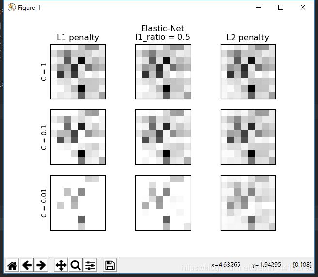
不同惩罚的稀疏度

import numpy as np
import matplotlib.pyplot as plt

from sklearn.linear_model import LogisticRegression
from sklearn import datasets
from sklearn.preprocessing import StandardScaler

# 加载数据
digits = datasets.load_digits()
X, y = digits.data, digits.target
# 标准化数据
X = StandardScaler().fit_transform(X)

# classify small against large digits
y = (y > 4).astype(np.int)      # 分为两类大于4和小于等于4

l1_ratio = 0.5  # L1 weight in the Elastic-Net regularization

fig, axes = plt.subplots(3, 3)

# Set regularization parameter
for i, (C, axes_row) in enumerate(zip((1, 0.1, 0.01), axes)):
    # turn down tolerance for short training time
    clf_l1_LR = LogisticRegression(C=C, penalty='l1', tol=0.01, solver='saga')
    clf_l2_LR = LogisticRegression(C=C, penalty='l2', tol=0.01, solver='saga')
    clf_en_LR = LogisticRegression(C=C, penalty='elasticnet', solver='saga',
                                   l1_ratio=l1_ratio, tol=0.01)
    clf_l1_LR.fit(X, y)
    clf_l2_LR.fit(X, y)
    clf_en_LR.fit(X, y)
    # 训练后的模型系数扁平化
    coef_l1_LR = clf_l1_LR.coef_.ravel()
    coef_l2_LR = clf_l2_LR.coef_.ravel()
    coef_en_LR = clf_en_LR.coef_.ravel()

    # coef_l1_LR contains zeros due to the
    # L1 sparsity inducing norm
    # 求稀疏度(零解的百分比)
    sparsity_l1_LR = np.mean(coef_l1_LR == 0) * 100
    sparsity_l2_LR = np.mean(coef_l2_LR == 0) * 100
    sparsity_en_LR = np.mean(coef_en_LR == 0) * 100
    # 打印当前的c值以及不同惩罚的稀疏度、得分
    print("C=%.2f" % C)
    print("{:<40} {:.2f}%".format("Sparsity with L1 penalty:", sparsity_l1_LR))
    print("{:<40} {:.2f}%".format("Sparsity with Elastic-Net penalty:",
                                  sparsity_en_LR))
    print("{:<40} {:.2f}%".format("Sparsity with L2 penalty:", sparsity_l2_LR))
    print("{:<40} {:.2f}".format("Score with L1 penalty:",
                                 clf_l1_LR.score(X, y)))
    print("{:<40} {:.2f}".format("Score with Elastic-Net penalty:",
                                 clf_en_LR.score(X, y)))
    print("{:<40} {:.2f}".format("Score with L2 penalty:",
                                 clf_l2_LR.score(X, y)))

    # 第一次绘图需要绘制横坐标
    if i == 0:
        axes_row[0].set_title("L1 penalty")
        axes_row[1].set_title("Elastic-Net\nl1_ratio = %s" % l1_ratio)
        axes_row[2].set_title("L2 penalty")
    # 绘制不同惩罚的稀疏度
    for ax, coefs in zip(axes_row, [coef_l1_LR, coef_en_LR, coef_l2_LR]):
        # 绘制灰度图
        ax.imshow(np.abs(coefs.reshape(8, 8)), interpolation='nearest',
                  cmap='binary', vmax=1, vmin=0)
        # 去掉横轴纵轴的刻度
        ax.set_xticks(())
        ax.set_yticks(())
    # 标注c值
    axes_row[0].set_ylabel('C = %s' % C)

plt.show()
1
2
3
4
5
6
7
8
9
10
11
12
13
14
15
16
17
18
19
20
21
22
23
24
25
26
27
28
29
30
31
32
33
34
35
36
37
38
39
40
41
42
43
44
45
46
47
48
49
50
51
52
53
54
55
56
57
58
59
60
61
62
63
64
65
66
67
68
69
70
71

正则化路径

iris = datasets.load_iris()
X = iris.data
y = iris.target

X = X[y != 2]
y = y[y != 2]

X /= X.max()  # Normalize X to speed-up convergence

# #############################################################################
# Demo path functions

cs = l1_min_c(X, y, loss='log') * np.logspace(0, 7, 16)


print("Computing regularization path ...")
start = time()  # 记录开始时间
# 构造逻辑回归对象  L1的正则化
# sag：即随机平均梯度下降，是梯度下降法的变种，和普通梯度下降法的区别是每次迭代仅仅用一部分的样本来计算梯度，
# 适合于样本数据多的时候，SAG是一种线性收敛算法，这个速度远比SGD快。
clf = linear_model.LogisticRegression(penalty='l1', solver='saga',
                                      tol=1e-6, max_iter=int(1e6),
                                      warm_start=True)
coefs_ = []     # 用于记录系数
# 用不同的c值进行训练
for c in cs:
    clf.set_params(C=c)
    clf.fit(X, y)
    coefs_.append(clf.coef_.ravel().copy())
# 运行时间
print("This took %0.3fs" % (time() - start))
# 16行4列的矩阵，第i行的4列表示第i次4个不同的系数
coefs_ = np.array(coefs_)
plt.plot(np.log10(cs), coefs_, marker='o')
ymin, ymax = plt.ylim()
plt.xlabel('log(C)')
plt.ylabel('Coefficients')
plt.title('Logistic Regression Path')
plt.axis('tight')
plt.show()
1
2
3
4
5
6
7
8
9
10
11
12
13
14
15
16
17
18
19
20
21
22
23
24
25
26
27
28
29
30
31
32
33
34
35
36
37
38
39
40