本站消息


Titanic
发布于2020-02-24 22:04 阅读(368) 评论(0) 点赞(7) 收藏(5)
导言:
这算是第一个真正意义上独立完成的Kaggle项目。期间参考了许多大神的做法,受益匪浅。本人技术不精,况且又是第一次做Kaggle的项目,请各位读者谅解,如有问题还请各位提出。谢谢大家的支持。
数据包与数据集导入
%matplotlib inline
import numpy as np
import pandas as pd
import matplotlib.pyplot as plt
import seaborn as sns
- 1
- 2
- 3
- 4
- 5
train = pd.read_csv('~/Coding/Kaggle/Titanic/train.csv')
test = pd.read_csv('~/Coding/Kaggle/Titanic/test.csv')
combine = pd.concat([train, test], sort = False, ignore_index=True)
PassengerId = test['PassengerId']
- 1
- 2
- 3
- 4
数据分析
概览
train.head()
- 1
| PassengerId | Survived | Pclass | Name | Sex | Age | SibSp | Parch | Ticket | Fare | Cabin | Embarked | |
|---|---|---|---|---|---|---|---|---|---|---|---|---|
| 0 | 1 | 0 | 3 | Braund, Mr. Owen Harris | male | 22.0 | 1 | 0 | A/5 21171 | 7.2500 | NaN | S |
| 1 | 2 | 1 | 1 | Cumings, Mrs. John Bradley (Florence Briggs Th... | female | 38.0 | 1 | 0 | PC 17599 | 71.2833 | C85 | C |
| 2 | 3 | 1 | 3 | Heikkinen, Miss. Laina | female | 26.0 | 0 | 0 | STON/O2. 3101282 | 7.9250 | NaN | S |
| 3 | 4 | 1 | 1 | Futrelle, Mrs. Jacques Heath (Lily May Peel) | female | 35.0 | 1 | 0 | 113803 | 53.1000 | C123 | S |
| 4 | 5 | 0 | 3 | Allen, Mr. William Henry | male | 35.0 | 0 | 0 | 373450 | 8.0500 | NaN | S |
我们不难看出,原始数据包括
PassengerId, Survived, Pclass, Name, Sex, Age, Sibsp, Parch, Ticket, Fare, Cabin, Embarked
这几个类目。
print(train.columns.values)
- 1
['PassengerId' 'Survived' 'Pclass' 'Name' 'Sex' 'Age' 'SibSp' 'Parch'
 'Ticket' 'Fare' 'Cabin' 'Embarked']
- 1
- 2
各类目数据类型和缺省值
接下来我们分析训练数据类目的类型以及其缺省值。
train.info()
- 1
<class 'pandas.core.frame.DataFrame'>
RangeIndex: 891 entries, 0 to 890
Data columns (total 12 columns):
PassengerId    891 non-null int64
Survived       891 non-null int64
Pclass         891 non-null int64
Name           891 non-null object
Sex            891 non-null object
Age            714 non-null float64
SibSp          891 non-null int64
Parch          891 non-null int64
Ticket         891 non-null object
Fare           891 non-null float64
Cabin          204 non-null object
Embarked       889 non-null object
dtypes: float64(2), int64(5), object(5)
memory usage: 83.6+ KB
- 1
- 2
- 3
- 4
- 5
- 6
- 7
- 8
- 9
- 10
- 11
- 12
- 13
- 14
- 15
- 16
- 17
test.info()
- 1
<class 'pandas.core.frame.DataFrame'>
RangeIndex: 418 entries, 0 to 417
Data columns (total 11 columns):
PassengerId    418 non-null int64
Pclass         418 non-null int64
Name           418 non-null object
Sex            418 non-null object
Age            332 non-null float64
SibSp          418 non-null int64
Parch          418 non-null int64
Ticket         418 non-null object
Fare           417 non-null float64
Cabin          91 non-null object
Embarked       418 non-null object
dtypes: float64(2), int64(4), object(5)
memory usage: 36.0+ KB
- 1
- 2
- 3
- 4
- 5
- 6
- 7
- 8
- 9
- 10
- 11
- 12
- 13
- 14
- 15
- 16
从上可以看出:
- train中,Age和Cabin有缺少
- test中,Age, Fare and Cabin有缺少
数据初步分析
继续分析
train.describe()
- 1
| PassengerId | Survived | Pclass | Age | SibSp | Parch | Fare | |
|---|---|---|---|---|---|---|---|
| count | 891.000000 | 891.000000 | 891.000000 | 714.000000 | 891.000000 | 891.000000 | 891.000000 |
| mean | 446.000000 | 0.383838 | 2.308642 | 29.699118 | 0.523008 | 0.381594 | 32.204208 |
| std | 257.353842 | 0.486592 | 0.836071 | 14.526497 | 1.102743 | 0.806057 | 49.693429 |
| min | 1.000000 | 0.000000 | 1.000000 | 0.420000 | 0.000000 | 0.000000 | 0.000000 |
| 25% | 223.500000 | 0.000000 | 2.000000 | 20.125000 | 0.000000 | 0.000000 | 7.910400 |
| 50% | 446.000000 | 0.000000 | 3.000000 | 28.000000 | 0.000000 | 0.000000 | 14.454200 |
| 75% | 668.500000 | 1.000000 | 3.000000 | 38.000000 | 1.000000 | 0.000000 | 31.000000 |
| max | 891.000000 | 1.000000 | 3.000000 | 80.000000 | 8.000000 | 6.000000 | 512.329200 |
通过上述结果,发现:
- PassengerId是unique的,与目标无关,在训练集中可以舍去
- 最终结果Survived是0,1表示的
- 很多人都没有直系亲属或旁系亲属
- 只有很少的人支付512美元的船票
- 登船人员的年龄普遍不是很大
我们首先将PassengerId条目在训练集中删去
紧接着,我们来观察非numeric的值
train.describe(include=['O'])# 注意,这个‘O’是 大写的‘o’,而不是数字0
- 1
| Name | Sex | Ticket | Cabin | Embarked | |
|---|---|---|---|---|---|
| count | 891 | 891 | 891 | 204 | 889 |
| unique | 891 | 2 | 681 | 147 | 3 |
| top | Ibrahim Shawah, Mr. Yousseff | male | CA. 2343 | C23 C25 C27 | S |
| freq | 1 | 577 | 7 | 4 | 644 |
发现:
- 乘客大部分为男士
- Ticket中有210张同样的票
- 大部分人从S港口登船
下面分析各类目与Survived之间的相互关系。
- Sex feature
观察男女的生存率差异
train[['Sex', 'Survived']].groupby('Sex', as_index=False).mean()\
.sort_values(by='Survived', ascending=False)
- 1
- 2
| Sex | Survived | |
|---|---|---|
| 0 | female | 0.742038 |
| 1 | male | 0.188908 |
女性的生存率普遍高于男性,Sex是较为重要的一个条目,需要保留。
- Pclass
train[['Pclass', 'Survived']].groupby('Pclass', as_index=False).mean()\
.sort_values(by='Survived', ascending=False)
- 1
- 2
| Pclass | Survived | |
|---|---|---|
| 0 | 1 | 0.629630 |
| 1 | 2 | 0.472826 |
| 2 | 3 | 0.242363 |
Pclass数值越小,生存几率越大。
- SibSp和Parch
train[['SibSp', 'Survived']].groupby('SibSp', as_index=False).mean()\
.sort_values(by='Survived', ascending=False)
- 1
- 2
| SibSp | Survived | |
|---|---|---|
| 1 | 1 | 0.535885 |
| 2 | 2 | 0.464286 |
| 0 | 0 | 0.345395 |
| 3 | 3 | 0.250000 |
| 4 | 4 | 0.166667 |
| 5 | 5 | 0.000000 |
| 6 | 8 | 0.000000 |
train[['Parch', 'Survived']].groupby('Parch', as_index=False).mean()\
.sort_values(by='Survived', ascending=False)
- 1
- 2
| Parch | Survived | |
|---|---|---|
| 3 | 3 | 0.600000 |
| 1 | 1 | 0.550847 |
| 2 | 2 | 0.500000 |
| 0 | 0 | 0.343658 |
| 5 | 5 | 0.200000 |
| 4 | 4 | 0.000000 |
| 6 | 6 | 0.000000 |
在这边其实可以考虑将Parch和SibSp合并成FamilySize
- Embarked
train[['Embarked', 'Survived']].groupby('Embarked', as_index=False).mean()\
.sort_values(by='Survived', ascending=False)
- 1
- 2
| Embarked | Survived | |
|---|---|---|
| 0 | C | 0.553571 |
| 1 | Q | 0.389610 |
| 2 | S | 0.336957 |
C港口登船的船员生存率最高
- Ticket
train[['Ticket', 'Survived']].groupby('Ticket', as_index=False).mean()\
.sort_values(by='Survived', ascending=False).head()
- 1
- 2
| Ticket | Survived | |
|---|---|---|
| 0 | 110152 | 1.0 |
| 180 | 26360 | 1.0 |
| 483 | 386525 | 1.0 |
| 479 | 382651 | 1.0 |
| 151 | 244373 | 1.0 |
关于登船人员的票证,因为特异值太多,可以考虑数据清洗时将其根据相同票证进行分组
- Age
由于Age是连续值,所以我们的分析通过图像来进行。
facet = sns.FacetGrid(train, hue='Survived', aspect=2)
facet.map(sns.kdeplot, 'Age', shade=True)
facet.set(xlim=(0, train['Age'].max()))
facet.add_legend()
plt.xlabel('Age')
plt.ylabel('density')
- 1
- 2
- 3
- 4
- 5
- 6
Text(12.359751157407416, 0.5, 'density')
- 1
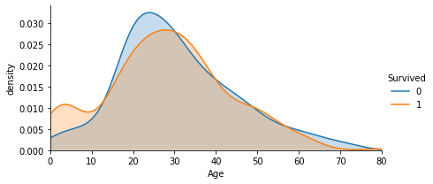
通过年龄-生存密度图可以看出,两曲线形状大部分重叠,只有在15岁以下生存率有差别。可以将年龄较低的部分单独分组。
- Fare
far = sns.FacetGrid(train, hue='Survived', aspect=2)
far.map(sns.kdeplot, 'Fare', shade=True)
far.set(xlim=(0, train['Fare'].max()))
far.add_legend()
plt.xlabel('Fare')
plt.ylabel('density')
- 1
- 2
- 3
- 4
- 5
- 6
Text(11.594234664351859, 0.5, 'density')
- 1
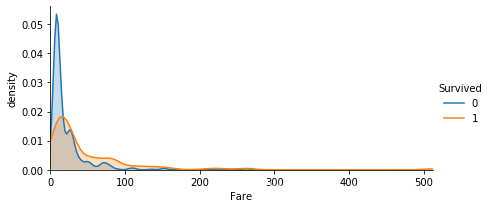
150之后的fare可以分为一组。0-25分组,25-100分组,100-150分组。
- Cabin
train['Cabin'].value_counts(dropna=True).head()
- 1
C23 C25 C27    4
B96 B98        4
G6             4
F2             3
D              3
Name: Cabin, dtype: int64
- 1
- 2
- 3
- 4
- 5
- 6
可以看出Cabin的数量非常多,在后面处理时会考虑只提取第一个字母来进行训练。
- Name
有关Name的这一部分将会在下面特征提取部分涉及。
特征提取
需要注意的是,接下来的特征提取以及数据清洗的阶段需要对整个数据集进行。
- FamilySize
将Parch和SibSp相加并加上1.
combine['FamilySize'] = combine['Parch'] + combine['SibSp'] + 1
combine = combine.drop(['Parch', 'SibSp'], axis=1)
- 1
- 2
处理完成之后我们再观察新创立的FamilySize。
sns.barplot(x='FamilySize', y='Survived', data=combine)
- 1
<matplotlib.axes._subplots.AxesSubplot at 0x1a25408668>
- 1
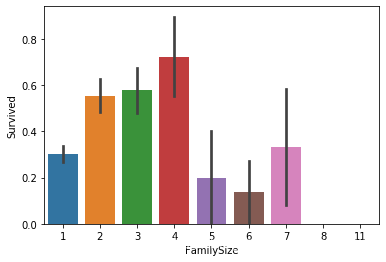
我们将FamilySize分成三组。
def fam(d):
    if (d>=2) & (d<=4):
        return 2
    elif ((d>4) & (d<=7)) | (d==1):
        return 1
    elif (d>7):
        return 0

combine['FamilyLabel'] = combine['FamilySize'].apply(fam)
sns.barplot(x='FamilyLabel', y='Survived', data=combine)
- 1
- 2
- 3
- 4
- 5
- 6
- 7
- 8
- 9
- 10
<matplotlib.axes._subplots.AxesSubplot at 0x1a25306860>
- 1
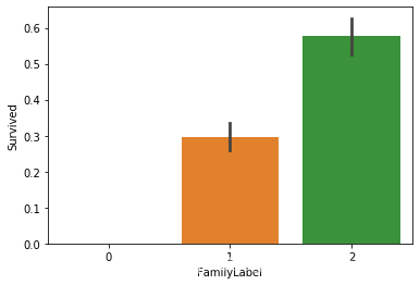
对FamilySize进行丢弃。
combine = combine.drop('FamilySize', axis=1)
- 1
- 对Cabin进行提取
首先将Cabin数据丢失的部分进行填充
combine['Cabin'] = combine['Cabin'].fillna('Unknown')
- 1
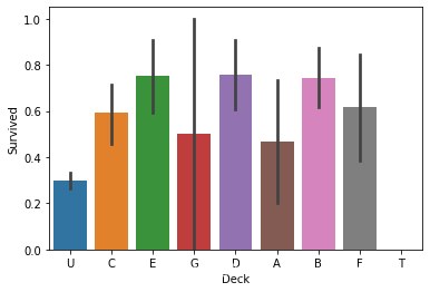
紧接着我们创建Deck属性,即对Cabin第一字母的提取。
combine['Deck'] = combine['Cabin'].str.get(0)
sns.barplot(x='Deck', y='Survived', data=combine)
- 1
- 2
<matplotlib.axes._subplots.AxesSubplot at 0x1a252dd898>
- 1
对Cabin进行丢弃。
combine = combine.drop('Cabin', axis=1)
- 1
将Deck进行分组。
deck_dict = {}
deck_dict.update(dict.fromkeys(['C', 'E', 'D', 'B', 'F'], 1))
deck_dict.update(dict.fromkeys(['U', 'G', 'A', 'T'], 0))

#combine['Deck'] = combine['Deck'].map(deck_dict)
#combine['Deck'] = combine['Deck'].astype(int)
- 1
- 2
- 3
- 4
- 5
- 6
- Ticket
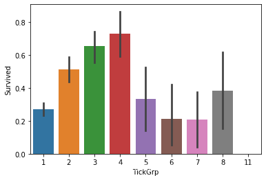
主要是对Ticket进行分组。
Tik_num = dict(combine['Ticket'].value_counts())
combine['TickGrp'] = combine['Ticket'].apply(lambda x: Tik_num[x])
sns.barplot(x='TickGrp', y='Survived', data=combine)
- 1
- 2
- 3
- 4
<matplotlib.axes._subplots.AxesSubplot at 0x1a24ab9940>
- 1
combine = combine.drop('Ticket', axis=1)
- 1
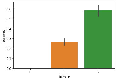
将TickGrp分成三组。
def tic(s):
    if (s>=2) & (s<=4):
        return 2
    elif ((s>4) & (s<=8)) | (s==1):
        return 1
    elif (s>8):
        return 0

combine['TickGrp'] = combine['TickGrp'].apply(tic)
sns.barplot(x='TickGrp', y='Survived', data=combine)
- 1
- 2
- 3
- 4
- 5
- 6
- 7
- 8
- 9
- 10
<matplotlib.axes._subplots.AxesSubplot at 0x1a256e7668>
- 1
- Name
具体某一位乘客的姓名肯定是和生存率无关。Name中有作用的成分应该是其中的Title。
下面提取出每个人的Title并创建新的Title条目。
combine['Title'] = combine['Name'].apply(lambda x: x.split(',')[1].split('.')[0].strip())
pd.crosstab(combine['Title'], combine['Survived'])
- 1
- 2
| Survived | 0.0 | 1.0 |
|---|---|---|
| Title | ||
| Capt | 1 | 0 |
| Col | 1 | 1 |
| Don | 1 | 0 |
| Dr | 4 | 3 |
| Jonkheer | 1 | 0 |
| Lady | 0 | 1 |
| Major | 1 | 1 |
| Master | 17 | 23 |
| Miss | 55 | 127 |
| Mlle | 0 | 2 |
| Mme | 0 | 1 |
| Mr | 436 | 81 |
| Mrs | 26 | 99 |
| Ms | 0 | 1 |
| Rev | 6 | 0 |
| Sir | 0 | 1 |
| the Countess | 0 | 1 |
combine = combine.drop('Name', axis=1)
- 1
我们需要将Title分类。
title_dict = {}
title_dict.update(dict.fromkeys(['Lady', 'the Countess','Capt', 'Col',\
 	'Don', 'Dr', 'Major', 'Rev', 'Sir', 'Jonkheer', 'Dona'], 'Rare'))
title_dict.update(dict.fromkeys(['Mlle'], 'Miss'))
title_dict.update(dict.fromkeys(['Ms'], 'Miss'))
title_dict.update(dict.fromkeys(['Mme'], 'Mrs'))
title_dict.update(dict.fromkeys(['Mr'], 'Mr'))
title_dict.update(dict.fromkeys(['Mrs'], 'Mrs'))
title_dict.update(dict.fromkeys(['Master'], 'Master'))

combine['Title'] = combine['Title'].map(title_dict)
combine[['Title', 'Survived']].groupby(['Title'], as_index=False).mean()\
.sort_values(by='Survived', ascending=False)
- 1
- 2
- 3
- 4
- 5
- 6
- 7
- 8
- 9
- 10
- 11
- 12
- 13
| Title | Survived | |
|---|---|---|
| 1 | Miss | 1.000000 |
| 3 | Mrs | 0.793651 |
| 0 | Master | 0.575000 |
| 4 | Rare | 0.347826 |
| 2 | Mr | 0.156673 |
title_mapping = {"Mr": 1, "Miss": 5, "Mrs": 4, "Master": 3, "Rare": 2}
combine['Title'] = combine['Title'].map(title_mapping)
combine['Title'] = combine['Title'].fillna(0)
- 1
- 2
- 3
- 把Sex转换为数字
combine['Sex'] = combine['Sex'].map( {'female': 1, 'male': 0} )
- 1
#combine.head()
- 1
数据清洗
- 将Embarked缺省值用众数填充
freq_port = combine.Embarked.dropna().mode()[0]
freq_port
- 1
- 2
'S'
- 1
combine['Embarked'] = combine['Embarked'].fillna(freq_port)
combine[['Embarked', 'Survived']].groupby(['Embarked'], as_index=False).mean()\
.sort_values(by='Survived', ascending=False)
- 1
- 2
- 3
| Embarked | Survived | |
|---|---|---|
| 0 | C | 0.553571 |
| 1 | Q | 0.389610 |
| 2 | S | 0.339009 |
#combine['Embarked'] = combine['Embarked'].map( {'S': 0, 'C': 1, 'Q': 2} )
combine.head()
- 1
- 2
| PassengerId | Survived | Pclass | Sex | Age | Fare | Embarked | FamilyLabel | Deck | TickGrp | Title | |
|---|---|---|---|---|---|---|---|---|---|---|---|
| 0 | 1 | 0.0 | 3 | male | 22.0 | 7.2500 | S | 2 | U | 1 | Mr |
| 1 | 2 | 1.0 | 1 | female | 38.0 | 71.2833 | C | 2 | C | 2 | Mrs |
| 2 | 3 | 1.0 | 3 | female | 26.0 | 7.9250 | S | 1 | U | 1 | NaN |
| 3 | 4 | 1.0 | 1 | female | 35.0 | 53.1000 | S | 2 | C | 2 | Mrs |
| 4 | 5 | 0.0 | 3 | male | 35.0 | 8.0500 | S | 1 | U | 1 | Mr |
- Fare
我们用Fare的平均数来填充Nan
combine['Fare'].fillna(combine['Fare'].dropna().median(), inplace=True)
combine.head()
- 1
- 2
| PassengerId | Survived | Pclass | Sex | Age | Fare | Embarked | FamilyLabel | Deck | TickGrp | Title | |
|---|---|---|---|---|---|---|---|---|---|---|---|
| 0 | 1 | 0.0 | 3 | male | 22.0 | 7.2500 | S | 2 | U | 1 | Mr |
| 1 | 2 | 1.0 | 1 | female | 38.0 | 71.2833 | C | 2 | C | 2 | Mrs |
| 2 | 3 | 1.0 | 3 | female | 26.0 | 7.9250 | S | 1 | U | 1 | NaN |
| 3 | 4 | 1.0 | 1 | female | 35.0 | 53.1000 | S | 2 | C | 2 | Mrs |
| 4 | 5 | 0.0 | 3 | male | 35.0 | 8.0500 | S | 1 | U | 1 | Mr |
创建FareBand
combine['FareBand'] = pd.qcut(combine['Fare'], 4)
combine[['FareBand', 'Survived']].groupby(['FareBand'], as_index=False).mean()\
.sort_values(by='FareBand', ascending=True)
- 1
- 2
- 3
| FareBand | Survived | |
|---|---|---|
| 0 | (-0.001, 7.896] | 0.197309 |
| 1 | (7.896, 14.454] | 0.303571 |
| 2 | (14.454, 31.275] | 0.441048 |
| 3 | (31.275, 512.329] | 0.600000 |
combine.loc[ combine['Fare'] <= 7.91, 'Fare'] = 0
combine.loc[(combine['Fare'] > 7.91) & (combine['Fare'] <= 14.454), 'Fare'] = 1
combine.loc[(combine['Fare'] > 14.454) & (combine['Fare'] <= 31), 'Fare']   = 2
combine.loc[ combine['Fare'] > 31, 'Fare'] = 3
combine['Fare'] = combine['Fare'].astype(int)
- 1
- 2
- 3
- 4
- 5
combine = combine.drop('FareBand', axis=1)
- 1
combine.head()
- 1
| PassengerId | Survived | Pclass | Sex | Age | Fare | Embarked | FamilyLabel | Deck | TickGrp | Title | |
|---|---|---|---|---|---|---|---|---|---|---|---|
| 0 | 1 | 0.0 | 3 | male | 22.0 | 0 | S | 2 | U | 1 | Mr |
| 1 | 2 | 1.0 | 1 | female | 38.0 | 3 | C | 2 | C | 2 | Mrs |
| 2 | 3 | 1.0 | 3 | female | 26.0 | 1 | S | 1 | U | 1 | NaN |
| 3 | 4 | 1.0 | 1 | female | 35.0 | 3 | S | 2 | C | 2 | Mrs |
| 4 | 5 | 0.0 | 3 | male | 35.0 | 1 | S | 1 | U | 1 | Mr |
- Age
因为Age的缺省值比较多,所以这边利用Sex, Title and Pclass三个特征值来构建随机森林模型,填充Age的缺失值。
from sklearn.ensemble import RandomForestRegressor
- 1
age = combine[['Age', 'Pclass', 'Sex', 'Title']]
age = pd.get_dummies(age)
kage = age[age.Age.notnull()].as_matrix()
ukage = age[age.Age.isnull()].as_matrix()
y = kage[:, 0]
X = kage[:, 1:]
rf = RandomForestRegressor(random_state=0, n_estimators=100, n_jobs=-1)
rf.fit(X, y)
P_age = rf.predict(ukage[:, 1::])
combine.loc[(combine.Age.isnull()), 'Age'] = P_age
- 1
- 2
- 3
- 4
- 5
- 6
- 7
- 8
- 9
- 10
/Users/helix/anaconda3/lib/python3.7/site-packages/ipykernel_launcher.py:3: FutureWarning: Method .as_matrix will be removed in a future version. Use .values instead.
  This is separate from the ipykernel package so we can avoid doing imports until
/Users/helix/anaconda3/lib/python3.7/site-packages/ipykernel_launcher.py:4: FutureWarning: Method .as_matrix will be removed in a future version. Use .values instead.
  after removing the cwd from sys.path.
- 1
- 2
- 3
- 4
combine.head()
- 1
| PassengerId | Survived | Pclass | Sex | Age | Fare | Embarked | FamilyLabel | Deck | TickGrp | Title | |
|---|---|---|---|---|---|---|---|---|---|---|---|
| 0 | 1 | 0.0 | 3 | male | 22.0 | 0 | S | 2 | U | 1 | Mr |
| 1 | 2 | 1.0 | 1 | female | 38.0 | 3 | C | 2 | C | 2 | Mrs |
| 2 | 3 | 1.0 | 3 | female | 26.0 | 1 | S | 1 | U | 1 | NaN |
| 3 | 4 | 1.0 | 1 | female | 35.0 | 3 | S | 2 | C | 2 | Mrs |
| 4 | 5 | 0.0 | 3 | male | 35.0 | 1 | S | 1 | U | 1 | Mr |
训练
特征转换
选取特征转换为数值变量。并且划分训练和测试集。
combine = combine[['Survived', 'Pclass', 'Sex', 'Age', 'Fare', 'Embarked', 'FamilyLabel',\
                   'Deck', 'TickGrp', 'Title']]
combine = pd.get_dummies(combine)
train = combine[combine['Survived'].notnull()]
test = combine[combine['Survived'].isnull()].drop('Survived', axis=1)
X = train.as_matrix()[:, 1:]
y = train.as_matrix()[:, 0]
- 1
- 2
- 3
- 4
- 5
- 6
- 7
/Users/helix/anaconda3/lib/python3.7/site-packages/ipykernel_launcher.py:6: FutureWarning: Method .as_matrix will be removed in a future version. Use .values instead.

/Users/helix/anaconda3/lib/python3.7/site-packages/ipykernel_launcher.py:7: FutureWarning: Method .as_matrix will be removed in a future version. Use .values instead.
  import sys
- 1
- 2
- 3
- 4
模型选择和参数优化
在这边偷懒,参考了他人的解答,直接选择随机森林模型。参数选择也没有使用GridSearchCV来选择。
from sklearn.pipeline import make_pipeline
from sklearn.feature_selection import SelectKBest
select = SelectKBest(k=20)
clf = RandomForestRegressor(random_state=10, warm_start=True,
                                   n_estimators=26,
                                   max_depth=6,
                                   max_features='sqrt')
pipeline = make_pipeline(select, clf)
pipeline.fit(X, y)
- 1
- 2
- 3
- 4
- 5
- 6
- 7
- 8
- 9
Pipeline(memory=None,
         steps=[('selectkbest',
                 SelectKBest(k=20,
                             score_func=<function f_classif at 0x1a21e462f0>)),
                ('randomforestregressor',
                 RandomForestRegressor(bootstrap=True, ccp_alpha=0.0,
                                       criterion='mse', max_depth=6,
                                       max_features='sqrt', max_leaf_nodes=None,
                                       max_samples=None,
                                       min_impurity_decrease=0.0,
                                       min_impurity_split=None,
                                       min_samples_leaf=1, min_samples_split=2,
                                       min_weight_fraction_leaf=0.0,
                                       n_estimators=26, n_jobs=None,
                                       oob_score=False, random_state=10,
                                       verbose=0, warm_start=True))],
         verbose=False)
- 1
- 2
- 3
- 4
- 5
- 6
- 7
- 8
- 9
- 10
- 11
- 12
- 13
- 14
- 15
- 16
- 17
获得结果并输出
pre=pipeline.predict(test)
def sss(d):
    if (d>=0.5):
        return 1
    elif (d<0.5):
        return 0
pre = pd.DataFrame(pre)
pre = pre[0].apply(sss)
- 1
- 2
- 3
- 4
- 5
- 6
- 7
- 8
sub=pd.DataFrame({"PassengerId": PassengerId, "Survived": pre.astype(np.int32)})
sub.to_csv('~/Coding/Kaggle/Titanic/res.csv', index=False)
- 1
- 2
- 3
参考:

所属网站分类: 技术文章 > 博客
作者:虎王168
链接:https://www.pythonheidong.com/blog/article/232296/265801ca7561df1e0b0e/
来源:python黑洞网
任何形式的转载都请注明出处,如有侵权 一经发现 必将追究其法律责任
7
0
收藏该文
昵称:
评论内容:(最多支持255个字符)
---无人问津也好,技不如人也罢,你都要试着安静下来,去做自己该做的事,而不是让内心的烦躁、焦虑,坏掉你本来就不多的热情和定力
站长公众号(new)
更多>
pdf(new)
更多>
问答(new)
更多>
游戏(new)
更多>