1.CIFAR-10数据集下载、解压

import urllib.request
import os
import tarfile
1
2
3

使用爬虫urlib库对网址 https://www.cs.toronto.edu/~kriz/cifar-10-python.tar.gz 内容进行下载；tarfile库对压缩文件解压。

#下载
url = 'https://www.cs.toronto.edu/~kriz/cifar-10-python.tar.gz'    #下载链接
filepath = 'data/cifar-10-python.tar.gz'                           #保存位置
if not os.path.exists(filepath):
    result = urllib.request.urlretrieve(url,filepath)    #函数爬取网址内容，并保存到filepath路径下
    print('downloaded:', result)
else:
    print('Date file already exists.')

#解压
if not os.path.exists("data/cifar-10-batches-py"):
    tfile = tarfile.open("data/cifar-10-python.tar.gz",'r:gz')
    result = tfile.extractall('data/')
    print('Extracted to ./data/cifar-10-batches-py/')
else:
    print('Directory already exists.')
1
2
3
4
5
6
7
8
9
10
11
12
13
14
15
16

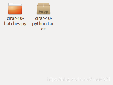
需要提前建好data目录，以存放下载内容。
解压后如下图：

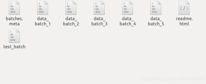
cifar-10-batches-py目录打开后如下:

2.处理数据

import os
import numpy as np
import pickle as p
import matplotlib.pyplot as plt
1
2
3
4

pickle可将文件的内容读出为对象，也可将对象内容写入文件保存。pickle.load()的参数还有点不清楚，以下两种参数设置都能将文件内容读出，但不知道二者的区别。

# 加载第i个batch
def load_CIFAR_batch(filename):
    with open(filename, 'rb') as f:
        
        # 一个样本由标签和图像数据组成
        data_dict = p.load(f, encoding='iso-8859-1')          # 按照官网格式取出，存放到字典中
        images = data_dict['data']
        labels = data_dict['labels']
        # 一个样本由标签和图像数据组成
        #         data_dict = p.load(f, encoding='bytes')     # 按照官网格式取出，存放到字典中
        #         images = data_dict[b'data']
        #         labels = data_dict[b'labels']
        #
        # 调整原始数据结构为 BCWH
        images = images.reshape(10000, 3, 32, 32)
        # tensorflow 处理图像数据的结构：BWHC
        # 把数据通道C移动到最后一个维度
        images = images.transpose(0, 2, 3, 1)

        labels = np.array(labels)
        return images, labels
1
2
3
4
5
6
7
8
9
10
11
12
13
14
15
16
17
18
19
20
21

load_CIFAR_batch 函数的返回值为一个batch的图像数据和标签。
原始的图像数据结构为：BCHW，batch、channel、width、high
而tensorflow处理图像的结构为BHWC，因此使用transpose函数改变数据shape。
transpose函数用法如下：
array([[0, 1, 2, 3],
[4, 5, 6, 7],
[8, 9, 10, 11]])

a.reshape(4, 3)
array([[0, 1, 2],
[3, 4, 5],
[6, 7, 8],
[9, 10, 11]])

a.transpose(1, 0)
array([[0, 4, 8],
[1, 5, 9],
[2, 6, 10],
[3, 7, 11]])

def load_CIFAR_data(data_dir):
    images_train = []
    labels_train = []
    for i in range(5):
        f = os.path.join(data_dir, 'data_batch_%d' % (i + 1))
        print('loading', f)
        # 调用load_CIFAR_batch()获得批量的图像及其对应的标签
        image_batch, label_batch = load_CIFAR_batch(f)
        images_train.append(image_batch)
        labels_train.append(label_batch)
        Xtrain = np.concatenate(images_train)
        Ytrain = np.concatenate(labels_train)
        del image_batch, label_batch

    Xtest, Ytest = load_CIFAR_batch(os.path.join(data_dir, 'test_batch'))
    print('finished loadding CIFAR-10 data')

    # 返回训练集的图像和标签，测试集的图像和标签
    return Xtrain, Ytrain, Xtest, Ytest
1
2
3
4
5
6
7
8
9
10
11
12
13
14
15
16
17
18
19

load_CIFAR_data 函数的返回值为整个训练集和测试集的图像和标签 Xtrain, Ytrain, Xtest, Ytest 。在for循环中依次访问data/cifar-10-batches-py/data_batch_i文件，从每个batch中取出数据，存入Xtrain, Ytrain中。最后从data/cifar-10-batches-py/test_batch取出测试集数据存入Xtest, Ytest 。

3.预处理

from sklearn.preprocessing import OneHotEncoder
from load_dataset import Xtrain, Ytrain, Xtest, Ytest
1
2

关于sklearn库的强大功能见其官方网站，在此运用了其对数据的预处理OneHot编码，调整lable数据形式。并加载上一部分处理结果。

# 将图像进行数字标准化
# Xtrain[0][0][0]
# array([59, 62, 63], dtype = unit8)-------进行归一化前的数据类型
Xtrain_normalize = Xtrain.astype('float32') / 255.0
Xtest_normalize = Xtest.astype('float32') / 255.0
# Xtrain_normalize[0][0][0]
# array([0.23137255, 0.24313726, 0.24705882], dtype = float32)-------进行归一化后的数据类型
1
2
3
4
5
6
7

对图像数据进行标准化，从array([59, 62, 63], dtype = unit8)–>array([0.23137255, 0.24313726, 0.24705882], dtype = float32)。

# 将标签数据进行标准化
# print(Ytrain.shape)
# (50000, )
# print(Ytrain[:5])-------显示前五个数据
# array([6,9,9,4,1])----------One-Hot编码前的标签数据
encoder = OneHotEncoder(sparse=False)
yy = [[0], [1], [2], [3], [4], [5], [6], [7], [8], [9]]
encoder.fit(yy)
Ytrain_reshape = Ytrain.reshape(-1, 1)
# 个参数为-1时,那么reshape函数会根据另一个参数的维度计算出数组的另外一个shape属性值,(-1, 1)就是将数据拆开为[[6], [9], [9],........ ]
Ytrain_onehot = encoder.transform(Ytrain_reshape)
Ytest_reshape = Ytest.reshape(-1, 1)
Ytest_onehot = encoder.transform(Ytest_reshape)
# print(Ytrain_onehot.shape)
# (50000, 10)
# print(Ytrain_onehot[:5])
# array([[0, 0, 0, 0, 0, 0, 1, 0, 0, 0],
#              [0, 0, 0, 0, 0, 0, 0, 0, 0, 1],
#      	    [0, 0, 0, 0, 0, 0, 0, 0, 0, 1],
#             [0, 0, 0, 0, 1, 0, 0, 0, 0, 0],
#            [0, 1, 0, 0, 0, 0, 0, 0, 0, 0]])
1
2
3
4
5
6
7
8
9
10
11
12
13
14
15
16
17
18
19
20
21

OneHot编码前后标签数据对比：
前：
print(Ytrain.shape)
–>> (50000, )
print(Ytrain[:5])
–>> array([6,9,9,4,1])
后：
print(Ytrain_onehot.shape)
–>> (50000, 10)
print(Ytrain_onehot[:5])
–>> array([[0, 0, 0, 0, 0, 0, 1, 0, 0, 0],
[0, 0, 0, 0, 0, 0, 0, 0, 0, 1],
[0, 0, 0, 0, 0, 0, 0, 0, 0, 1],
[0, 0, 0, 0, 1, 0, 0, 0, 0, 0],
[0, 1, 0, 0, 0, 0, 0, 0, 0, 0]])

4.构建网络结构

import tensorflow as tf
# tf.reset_default_graph()
tf.compat.v1.reset_default_graph
1
2
3

# 定义共享参数
# 定义权值
def weight(shape):
    # 在构建模型时，需要使用tf.Variable来创建一个变量,在训练时这个变量不断更新
    # 使用函数tf.truncated_normal(截断的正态分布)来生成标准差为0.1的随机数来初始化权值
    return tf.Variable(tf.random.truncated_normal(shape, stddev=0.1), name='W')

# 定义偏置，初始化为0.1
def bias(shape):
    return tf.Variable(tf.constant(0.1, shape=shape), name='b')

# 定义卷积操作,步长为1,padding为‘SAME’
def conv2d(x, W):
    # tf.nn.conv2d(input, filter, strides, padding, use_cudnn_on_gpu=None, name=None)
    return tf.nn.conv2d(x, W, strides=[1, 1, 1, 1], padding='SAME')

# 定义池化操作,步长为2,及原尺寸的长宽各除以2
def max_pool_2x2(x):
    # tf.nn.max_pool(value, ksize, strides, padding, name=None)
    return tf.nn.max_pool2d(x, ksize=[1, 2, 2, 1], strides=[1, 2, 2, 1], padding='SAME')
1
2
3
4
5
6
7
8
9
10
11
12
13
14
15
16
17
18
19
20

下面开始构建图：

name_scope ‘input_layer’:
第一层输入使用占位符placeholder产生第一个节点。

name_scope ‘conv_1’:
在此命名空间内生成变量weight和bias，命名为’W’和’b’，生成卷积操作节点，relu操作节点。

name_scope ‘pool_1’:
在此命名空间内生成池化操作节点。

name_scope ‘conv_2’:
在此命名空间内生成变量weight和bias，命名为’W’和’b’，生成卷积操作节点，relu操作节点。

name_scope ‘pool_2’:
在此命名空间内生成池化操作节点。

name_scope ‘fc’:
在此命名空间内生成变量weight和bias，命名为’W’和’b’，生成reshape操作节点，relu操作节点，dropout操作节点。

name_scope ‘output_layer’:
在此命名空间内生成变量weight和bias，命名为’W’和’b’，生成softmax操作。

name_scope ‘optimizer’:
在此命名空间内使用占位符placeholder产生一个输出y节点，定义计算损失和优化操作。

name_scope ‘evalution’:
在此命名空间内定义求得准确率操作。

# 这里的name_scope是创建了一个命名空间，相当于一个参数名称空间，这个空间conv_1里存储了许多参数：W1 b1  conv_1

# 定义网络结构
# 输入层,32x32图像，3通道RGB
with tf.name_scope('input_layer'):
    x = tf.compat.v1.placeholder('float', shape=[None, 32, 32, 3], name="x")

# 第1个卷积层
# 输入通道：3，输出通道：32，卷积后图像尺寸不变，依然是32x32
with tf.name_scope('conv_1'):
    W1 = weight([3, 3, 3, 32])  # [k_width, k_heigth, input_chn, output_chn]
    b1 = bias([32])  # 与output_chn一致
    conv_1 = conv2d(x, W1) + b1
    conv_1 = tf.nn.relu(conv_1)

# 第一个池化层
# 将32x32图像缩小为16x16，池化不改变通道数量，依旧是32个
with tf.name_scope('pool_1'):
    pool_1 = max_pool_2x2(conv_1)

# 第2个卷积层
# 输入通道：32，输出通道：64，卷积后图像尺寸不变，依旧是16x16
with tf.name_scope('conv_2'):
    W2 = weight([3, 3, 32, 64])
    b2 = bias([64])
    conv_2 = conv2d(pool_1, W2) + b2
    conv_2 = tf.nn.relu(conv_2)

# 第二个池化层
# 将16x16图像缩小为8x8，池化不改变通道数量，依旧是64个
with tf.name_scope('poll_2'):
    pool_2 = max_pool_2x2(conv_2)

# 全连接层
# 将第2个池化层的64个8x8的图像转化为一维向量，长度是64*8*8=4096
# 选用128个神经元
with tf.name_scope('fc'):
    W3 = weight([4096, 128])
    b3 = bias([128])
    flat = tf.reshape(pool_2, [-1, 4096])
    h = tf.nn.relu(tf.matmul(flat, W3) + b3)
    h_dropout = tf.nn.dropout(h, rate=0.2)

# 输出层
# 输出层共有10个神经元，对应到0～9这10个类别
with tf.name_scope('output_layer'):
    W4 = weight([128, 10])
    b4 = bias([10])
    pred = tf.nn.softmax(tf.matmul(h_dropout, W4) + b4)

# 构建模型
with tf.name_scope("optimizer"):
    # 定义占位符
    y = tf.compat.v1.placeholder("float", shape=[None, 10], name="label")
    # 定义损失函数
    loss_function = tf.reduce_mean(tf.nn.softmax_cross_entropy_with_logits(logits=pred, labels=y))
    # 选择优化器
    optimizer = tf.train.AdamOptimizer(learning_rate=0.0001).minimize(loss_function)

# 定义准确率
with tf.name_scope("evalution"):
    correct_prediction = tf.equal(tf.argmax(pred, 1), tf.argmax(y, 1))
    accuracy = tf.reduce_mean(tf.cast(correct_prediction, "float"))
1
2
3
4
5
6
7
8
9
10
11
12
13
14
15
16
17
18
19
20
21
22
23
24
25
26
27
28
29
30
31
32
33
34
35
36
37
38
39
40
41
42
43
44
45
46
47
48
49
50
51
52
53
54
55
56
57
58
59
60
61
62
63

网络结构为：输入层–>卷积层–>池化层–>卷积层–>池化层–>全连接层–>输出层
通道数：3–>32–>32–>64–>64–>一维向量4096

5.开始训练

加载所需库和前几个包

import os
import tensorflow as tf
from preprocess import Xtrain_normalize, Xtest_normalize, Ytrain_onehot, Ytest_onehot
from time import time
from load_dataset import Xtrain, Ytrain, Xtest, Ytest
import network_stucture as ns
import matplotlib.pyplot as plt
1
2
3
4
5
6
7

运行时一直有如下提醒错误，查找资料后加入以下代码，问题解决。

from tensorflow.compat.v1 import ConfigProto
from tensorflow.compat.v1 import InteractiveSession

config = ConfigProto()
config.gpu_options.allow_growth = True
session = InteractiveSession(config=config)
# 意思是对GPU进行按需分配。
# 主要原因是我的图像比较大，消耗GPU资源较多。这个错误提示有很大的误导性，让人一直纠结CUDA和CuDNN的版本问题。故在此立贴，以免后人重蹈覆辙。
1
2
3
4
5
6
7
8

设置train_epochs和batch_size分别为25和50，建立存放accuracy和loss的列表。开启一个session，开始训练。

train_epochs = 25
batch_size = 50
total_batch = int(len(Xtrain) / batch_size)
epoch_list = []
accuracy_list = []
loss_list = []

epoch = tf.Variable(0, name='epoch', trainable=False)

startTime = time()

sess = tf.compat.v1.Session()
init = tf.compat.v1.global_variables_initializer()
sess.run(init)

# 断点续训
# 设置检查点存储目录
ckpt_dir = "CIFAR_log/"
if not os.path.exists(ckpt_dir):
    os.makedirs(ckpt_dir)
1
2
3
4
5
6
7
8
9
10
11
12
13
14
15
16
17
18
19
20
21

用tf.train.Saver()创建一个Saver来管理模型中的所有变量。

# 生成saver
saver = tf.train.Saver(max_to_keep=1)

# 如果有检查点文件，读取最新检查点文件，恢复各种变量值
ckpt = tf.train.latest_checkpoint(ckpt_dir)
if ckpt != None:
    saver.restore(sess, ckpt)  # 加载所有参数
    # 从这里开始就可以直接使用模型进行预测，或者接着继续训练了
else:
    print("Training from scratch")

# 获取续训参数
start = sess.run(epoch)
print("Training starts from {} epoch.".format(start + 1))


# 迭代训练
def get_train_batch(number, batch_size):
    return Xtrain_normalize[number * batch_size:(number + 1) * batch_size], \
           Ytrain_onehot[number * batch_size:(number + 1) * batch_size]


for ep in range(start, train_epochs):

    for i in range(total_batch):
        batch_x, batch_y = get_train_batch(i, batch_size)
        sess.run(ns.optimizer, feed_dict={ns.x: batch_x, ns.y: batch_y})
        if i % 100 == 0:
            print("Step{}".format(i), "finished")
    loss, acc = sess.run([ns.loss_function, ns.accuracy], feed_dict={ns.x: batch_x, ns.y: batch_y})
    epoch_list.append(ep + 1)
    loss_list.append(loss)
    accuracy_list.append(acc)

    print("Train epoch:", '%02d' % (sess.run(epoch) + 1), "Loss=", "{:.6f}".format(loss), "Accuracy=", acc)

    # 保存检查点
    saver.save(sess, ckpt_dir + "CIFAR10_cnn_model.cpkt", global_step=ep + 1)
    sess.run(epoch.assign(ep + 1))

duration = time() - startTime
print("Train finished takes:", duration)
1
2
3
4
5
6
7
8
9
10
11
12
13
14
15
16
17
18
19
20
21
22
23
24
25
26
27
28
29
30
31
32
33
34
35
36
37
38
39
40
41
42

创建目录存放loss和accuracy的历史值列表。

diir = "LOSS&ACC/"
if not os.path.exists(diir):
    os.makedirs(diir)
aimPath = os.path.dirname(diir) + "/tempPickle.pkl"

# 写入
with open(aimPath, "wb") as f:
    pickle.dump(accuracy_list, f)
    pickle.dump(loss_list, f)
    pickle.dump(epoch_list, f)
1
2
3
4
5
6
7
8
9
10

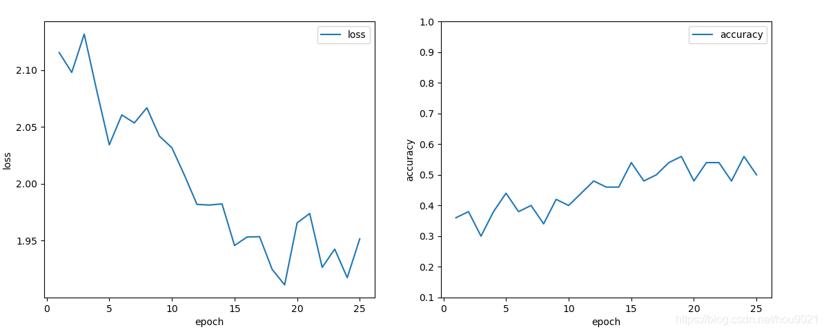
使loss和accuracy可视化显示。

import os
import matplotlib.pyplot as plt
import pickle

diir = "LOSS&ACC/"
if not os.path.exists(diir):
    os.makedirs(diir)
aimPath = os.path.dirname(diir) + "/tempPickle.pkl"

# 读取
with open(aimPath, "rb") as f:
    accuracy_list = pickle.load(f)
    loss_list = pickle.load(f)
    epoch_list = pickle.load(f)

fig = plt.figure()

plt.subplot(1, 2, 1)
# 可视化损失值
plt.plot(epoch_list, loss_list, label="loss")
fig = plt.gcf()
fig.set_size_inches(10, 5)
plt.ylabel('loss')
plt.xlabel('epoch')
plt.legend(['loss'], loc='upper right')

plt.subplot(1, 2, 2)
# 可视化准确率
plt.plot(epoch_list, accuracy_list, label="accuracy")
fig = plt.gcf()
fig.set_size_inches(10, 5)
plt.ylim(0.1, 1)
plt.ylabel('accuracy')
plt.xlabel('epoch')
plt.legend()
plt.show()

1
2
3
4
5
6
7
8
9
10
11
12
13
14
15
16
17
18
19
20
21
22
23
24
25
26
27
28
29
30
31
32
33
34
35
36
37

5.训练过程

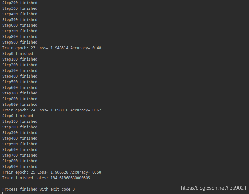
得到最终的loss和accuracy值。

6.可视化结果