优化与深度学习

优化与估计

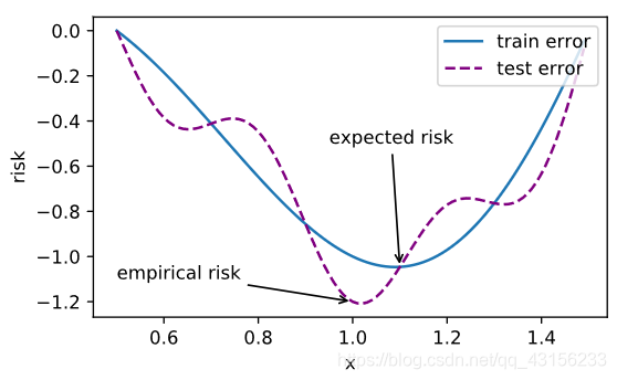
尽管优化方法可以最小化深度学习中的损失函数值，但本质上优化方法达到的目标与深度学习的目标并不相同。
优化方法目标：训练集损失函数值
深度学习目标：测试集损失函数值（泛化性）

%matplotlib inline
import sys
sys.path.append('/home/kesci/input')
import d2lzh1981 as d2l
from mpl_toolkits import mplot3d # 三维画图
import numpy as np
1
2
3
4
5
6

def f(x): return x * np.cos(np.pi * x)
def g(x): return f(x) + 0.2 * np.cos(5 * np.pi * x)

d2l.set_figsize((5, 3))
x = np.arange(0.5, 1.5, 0.01)
fig_f, = d2l.plt.plot(x, f(x),label="train error")
fig_g, = d2l.plt.plot(x, g(x),'--', c='purple', label="test error")
fig_f.axes.annotate('empirical risk', (1.0, -1.2), (0.5, -1.1),arrowprops=dict(arrowstyle='->'))
fig_g.axes.annotate('expected risk', (1.1, -1.05), (0.95, -0.5),arrowprops=dict(arrowstyle='->'))
d2l.plt.xlabel('x')
d2l.plt.ylabel('risk')
d2l.plt.legend(loc="upper right")
1
2
3
4
5
6
7
8
9
10
11
12

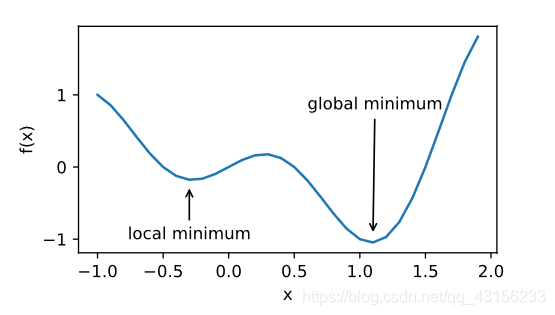
优化在深度学习中的挑战

1. 局部最小值
2. 鞍点
3. 梯度消失
   

def f(x):
    return x * np.cos(np.pi * x)

d2l.set_figsize((4.5, 2.5))
x = np.arange(-1.0, 2.0, 0.1)
fig,  = d2l.plt.plot(x, f(x))
fig.axes.annotate('local minimum', xy=(-0.3, -0.25), xytext=(-0.77, -1.0),
                  arrowprops=dict(arrowstyle='->'))
fig.axes.annotate('global minimum', xy=(1.1, -0.95), xytext=(0.6, 0.8),
                  arrowprops=dict(arrowstyle='->'))
d2l.plt.xlabel('x')
d2l.plt.ylabel('f(x)');
1
2
3
4
5
6
7
8
9
10
11
12

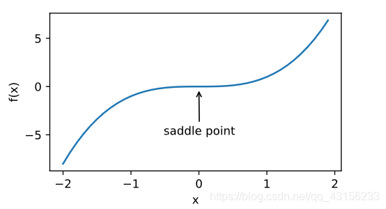
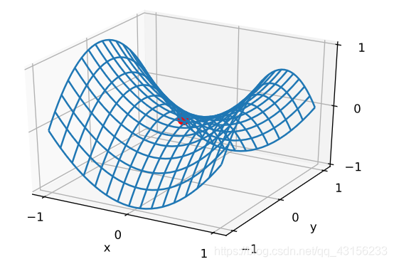
鞍点

x = np.arange(-2.0, 2.0, 0.1)
fig, = d2l.plt.plot(x, x**3)
fig.axes.annotate('saddle point', xy=(0, -0.2), xytext=(-0.52, -5.0),
                  arrowprops=dict(arrowstyle='->'))
d2l.plt.xlabel('x')
d2l.plt.ylabel('f(x)');
1
2
3
4
5
6

x, y = np.mgrid[-1: 1: 31j, -1: 1: 31j]
z = x**2 - y**2

d2l.set_figsize((6, 4))
ax = d2l.plt.figure().add_subplot(111, projection='3d')
ax.plot_wireframe(x, y, z, **{'rstride': 2, 'cstride': 2})
ax.plot([0], [0], [0], 'ro', markersize=10)
ticks = [-1,  0, 1]
d2l.plt.xticks(ticks)
d2l.plt.yticks(ticks)
ax.set_zticks(ticks)
d2l.plt.xlabel('x')
d2l.plt.ylabel('y');
1
2
3
4
5
6
7
8
9
10
11
12
13

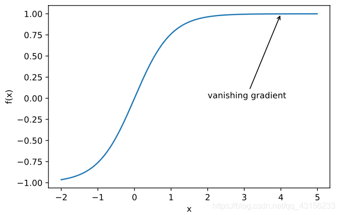
梯度消失

x = np.arange(-2.0, 5.0, 0.01)
fig, = d2l.plt.plot(x, np.tanh(x))
d2l.plt.xlabel('x')
d2l.plt.ylabel('f(x)')
fig.axes.annotate('vanishing gradient', (4, 1), (2, 0.0) ,arrowprops=dict(arrowstyle='->'))
1
2
3
4
5

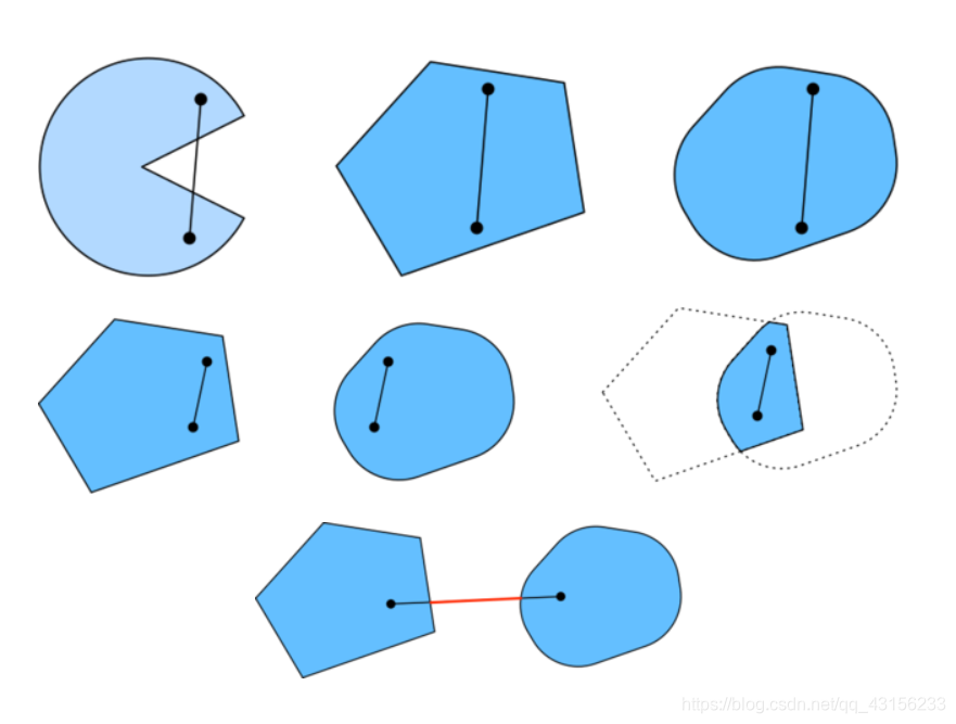
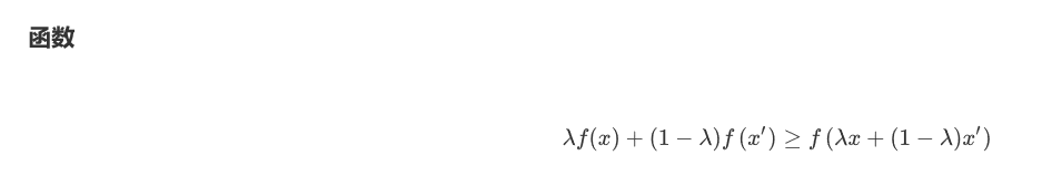
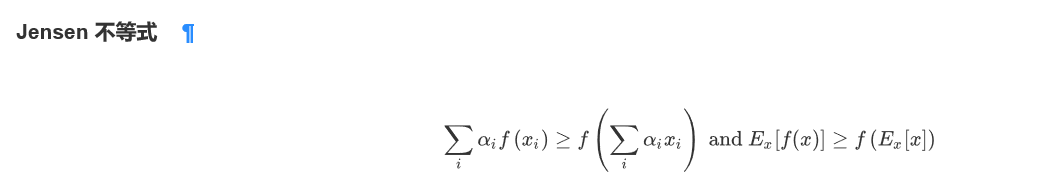
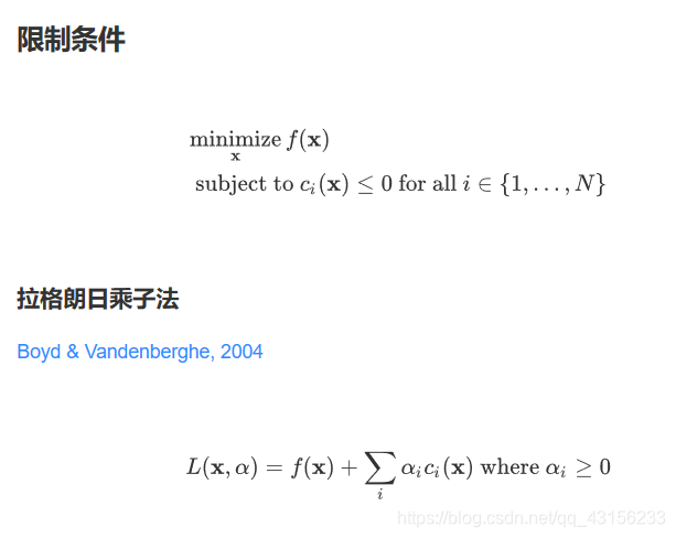
凸性 （Convexity）

基础

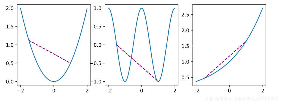
集合

def f(x):
    return 0.5 * x**2  # Convex

def g(x):
    return np.cos(np.pi * x)  # Nonconvex

def h(x):
    return np.exp(0.5 * x)  # Convex

x, segment = np.arange(-2, 2, 0.01), np.array([-1.5, 1])
d2l.use_svg_display()
_, axes = d2l.plt.subplots(1, 3, figsize=(9, 3))

for ax, func in zip(axes, [f, g, h]):
    ax.plot(x, func(x))
    ax.plot(segment, func(segment),'--', color="purple")
    # d2l.plt.plot([x, segment], [func(x), func(segment)], axes=ax)
1
2
3
4
5
6
7
8
9
10
11
12
13
14
15
16
17

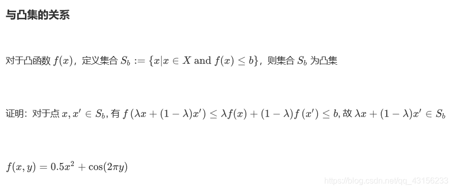
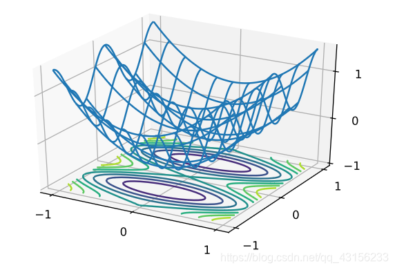
x, y = np.meshgrid(np.linspace(-1, 1, 101), np.linspace(-1, 1, 101),
                   indexing='ij')

z = x**2 + 0.5 * np.cos(2 * np.pi * y)

# Plot the 3D surface
d2l.set_figsize((6, 4))
ax = d2l.plt.figure().add_subplot(111, projection='3d')
ax.plot_wireframe(x, y, z, **{'rstride': 10, 'cstride': 10})
ax.contour(x, y, z, offset=-1)
ax.set_zlim(-1, 1.5)

# Adjust labels
for func in [d2l.plt.xticks, d2l.plt.yticks, ax.set_zticks]:
    func([-1, 0, 1])
1
2
3
4
5
6
7
8
9
10
11
12
13
14
15

凸函数与二阶函数

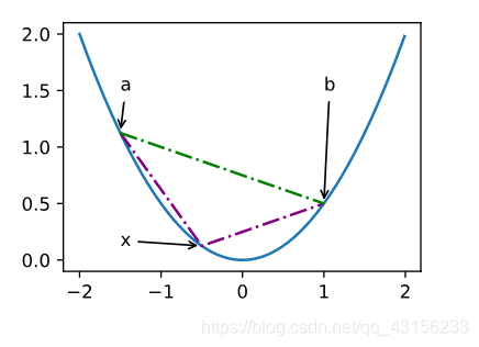
def f(x):
    return 0.5 * x**2

x = np.arange(-2, 2, 0.01)
axb, ab = np.array([-1.5, -0.5, 1]), np.array([-1.5, 1])

d2l.set_figsize((3.5, 2.5))
fig_x, = d2l.plt.plot(x, f(x))
fig_axb, = d2l.plt.plot(axb, f(axb), '-.',color="purple")
fig_ab, = d2l.plt.plot(ab, f(ab),'g-.')

fig_x.axes.annotate('a', (-1.5, f(-1.5)), (-1.5, 1.5),arrowprops=dict(arrowstyle='->'))
fig_x.axes.annotate('b', (1, f(1)), (1, 1.5),arrowprops=dict(arrowstyle='->'))
fig_x.axes.annotate('x', (-0.5, f(-0.5)), (-1.5, f(-0.5)),arrowprops=dict(arrowstyle='->'))
1
2
3
4
5
6
7
8
9
10
11
12
13
14