Topic：表情识别
Env： win10 + Pycharm2018 + Python3.6.8
Date: Date: 2019/6/23~25 by hw_Chen2018
【感谢参考文献作者的辛苦付出；编写不易，转载请注明出处，感谢！】
一.简要介绍
本文方法参考文献【1】的表情识别方法，实验数据集为JAFFE，实验方法较为传统：手工设计特征+浅层分类器，选择常规的划分训练集与测试方法：70%训练集、30%测试集。最后识别正确率73%，比不上目前深度学习方法，想要学习深度学习的朋友，抱歉本文不能提供任何帮助，不过做为Gabor滤波器的学习，可以作为参考。
二.数据集
实验中采用Jaffe数据库，数据库中包含了213幅（每幅图像的分辨率：256像素×256像素）日本女性的脸相，每幅图像都有原始的表情定义。表情库中共有10个人，每个人有7种表情（中性脸、高兴、悲伤、惊奇、愤怒、厌恶、恐惧）。JAFFE数据库均为正面脸相，且把原始图像进行重新调整和修剪，使得眼睛在数据库图像中的位置大致相同，脸部尺寸基本一致，光照均为正面光源，但光照强度有差异。【2】
三.Gabor滤波器
Gabor小波与人类视觉系统中简单细胞的视觉刺激响应非常相似。Gabor小波对于图像的边缘敏感，能够提供良好的方向选择和尺度选择特性，而且对于光照变化不敏感,能够提供对光照变化良好的适应性。因此Gabor小波被广泛应用于视觉信息理解。
在空域，一个2维的Gabor滤波器是一个正弦平面波和高斯核函数的乘积。【2】


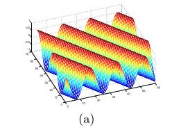
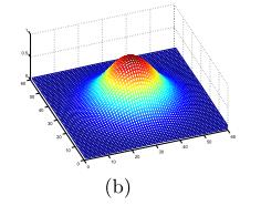
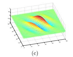
Gabor滤波器的表达式如下：

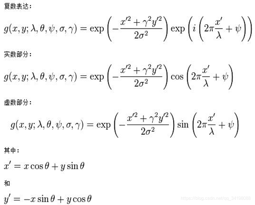
每个参数的意义以及对比图，可参考【3】
三.实验过程
1.数据库中灰度图分辨率是256256，实验中所用到的是进过裁剪的人脸图像，大小为4848。
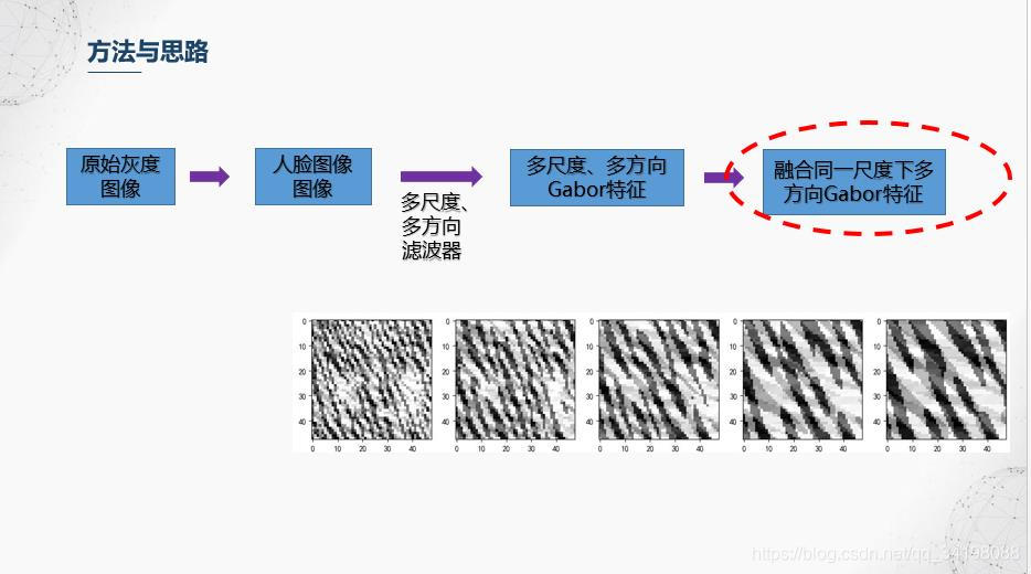
2.构建多尺度、多方向Gabor滤波器，实验中构建的滤波器尺度为5，方向数为8，下图就是所构建的Gabor滤波。值得注意的是通过Gabor滤波得到的结果是一个复数，在实验中只选用了实部进行实验，后面展示的一些结果图都是结果的实部。

3.人脸多尺度多方向特征

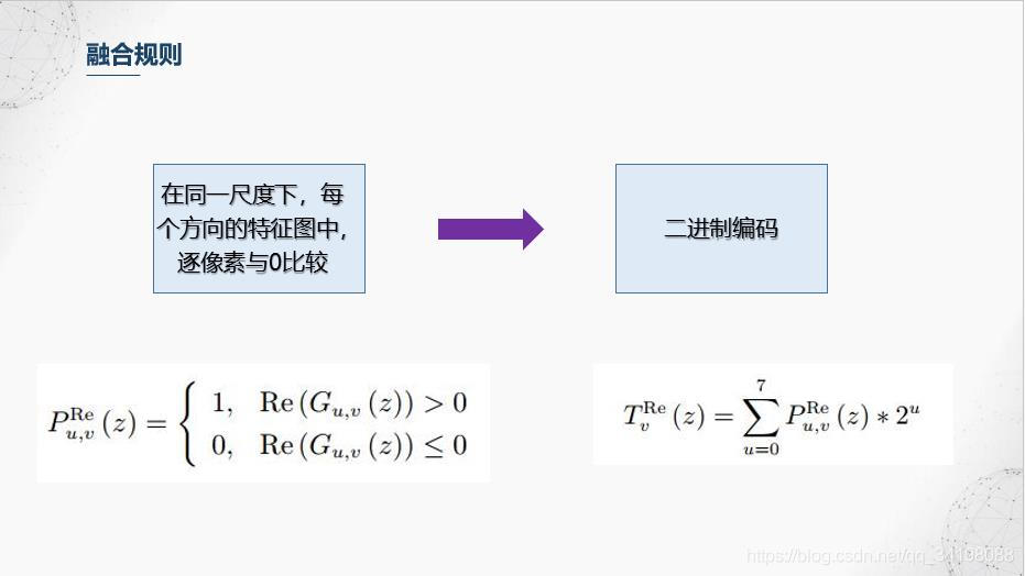
4.我们前面得到了5个尺度，8个方向的Gabor特征图，融合规则是对每个尺度进行操作，融合的第一步是，在同一尺度下，每个方向的特征图中，逐像素与0比较，大于0的置1，小于等于0置0，之后对每个像素进行二进制编码，在右边公式中，u代表方向序号，v代表尺度，对于融合后的图像的每个像素，它等于每个方向的的二进制编码之和。更多融合方法可查阅文献【1】。



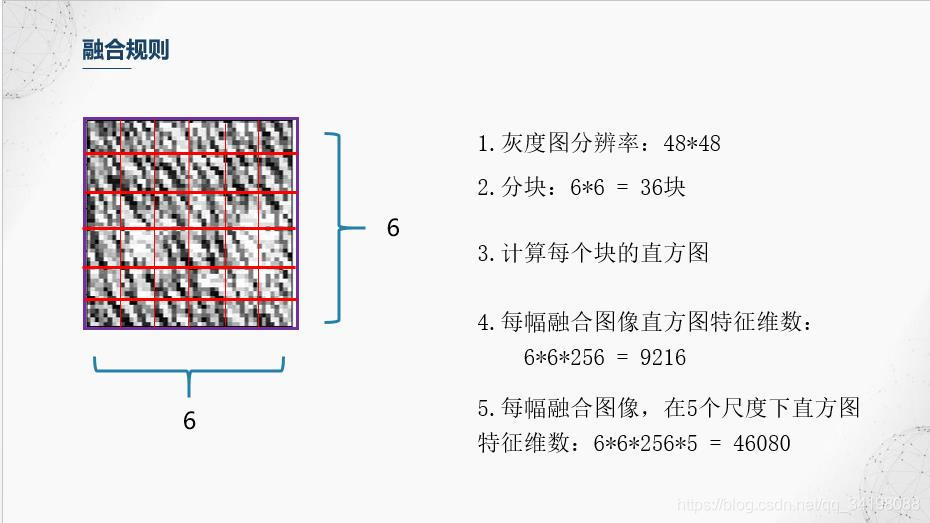
5.分块直方图
前面滤波器也提到，Gabor滤波器具有很好的局部特性和方向特性，而图像直方图从图像整体分布角度考虑，反映了图像的统计特性，但是却丢失了图像结构特性，因此【1】中避免使用全局图像直方图，采用分块直方图的方法，即保持了Gabor的局部细节，又保持了一定的结构特性。本文划分成36个小块。


6.降维与分类器训练
由于经过分块直方图后特征维数46080，相对于共213个样本的JAFFE数据集来说，维数偏高，同时也存在特征冗余，即并不是所有特征都对分类起积极作用，这里使用比较简单的PCA进行降维和特征选择，感兴趣的朋友可以搜下其他的特征选择，比如常用的包裹式、过滤式等等的特征选择方法以及以流形学习为代表的非线性降维方法等等。选择前13个主成分，贡献率达到90%。使用随机森林进行分类。

四.实验结果与分析
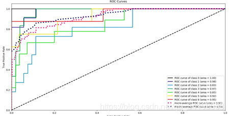
ROC曲线

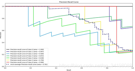
PR曲线

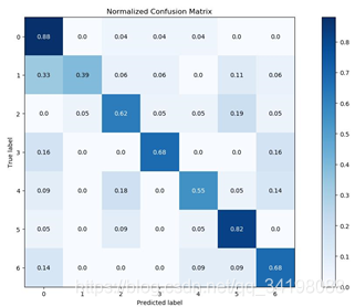
混淆矩阵

(1)对于实验中使用的特征提取及构建的分类器，通过ROC曲线可知，各类别中分类准确率最高的是第一类，对于测试集全部分类正确，其AUC等于1；分类正确率最低是第三类，低于平均正确率，其AUC等于0.83。
(2) 对于实验中使用的特征提取及构建的分类器，通过PR曲线可知，各类别中分类准确率最高的仍然是第一类，对于测试集全部分类正确，PR曲线面积等于1；分类正确率最低仍然是第三类，同样低于平均正确率，PR曲线面积等于0.584。
(3)通过混线矩阵可以很直观看出，分类器容易把第二类分成第一类，分类结果最好的仍然是第一类。

五.实验代码
1.提取特征并保存在CSV文件中。(部分代码参考了OpenCV中Gabor滤波器)

# coding:utf-8
# ------------------------------------
# topic: discrete express recognition
# method: Gabor Multi-orientation Features Fusion and Block Histogram  +  random forest
# source: 刘帅师等: 基于 Gabor 多方向特征融合与分块直方图的人脸表情识别方法 等
# env: win10 + pycharm + Python3.6.8
# date: 2019/6/21~25
# author: Chen_hw
# CSDN：https://blog.csdn.net/qq_34198088
# 编写不易，转载请注明出处！
# ------------------------------------
import numpy as np
import pandas as pd
import matplotlib.pyplot as plt
import cv2
from scipy import signal
import matplotlib
import time
import csv
matplotlib.rcParams['font.sans-serif'] = ['SimHei']
matplotlib.rcParams['font.family'] = 'sans-serif'
matplotlib.rcParams['axes.unicode_minus'] = False

class DiscreteAffectModel(object):
    def __init__(self, dataset_path):
        self.emotion ={0:'Angry', 1:'Disgust', 2:'Fear', 3:'Happy', 4:'Sad', 5:'Surprise', 6:'Neutral'}
        self.path = dataset_path
        self.gabor_filter_size = [50, 50]
        self.gabor_filter_lambda = [2*np.power(2, 0.5),
                                    3*np.power(2, 0.5),
                                    4*np.power(2, 0.5),
                                    5*np.power(2, 0.5),
                                    6*np.power(2, 0.5)]                 # 正弦因子波长。通常大于等于2.但不能大于输入图像尺寸的五分之一
        self.gabor_filter_sigma = [1.58,
                                   2.38,
                                   3.17,
                                   3.96,
                                   4.75]                                # 高斯包络的标准差.带宽设置为1时，σ 约= 0.56 λ
        self.gabor_filter_theta = [theta for theta in np.arange(0, np.pi, np.pi / 8) ]  # Gabor函数平行条纹的法线方向
        self.gabor_filter_gamma = 0.5                                   # 空间纵横比
        self.gabor_filter_psi = 0                                       # 相移
        self.filters_real = []                                          # 滤波器实数部分
        self.filters_imaginary = []                                     # 滤波器虚数部分
        self.filtering_result_real_component = []
        self.load_dataset()
        self.build_gabor_filter()
        # self.show_gabor_filters()
        # self.show_different_gabor_filteringResult()
        # self.show_fusion_rule_1_result()
        self.process_images()


        # a = np.array([[1,2,3,4,5,6,7,8],
        #               [1,2,3,4,5,6,7,8],
        #               [1,2,3,4,5,6,7,8],
        #               [1,2,3,4,5,6,7,8],
        #               [1,2,3,4,5,6,7,8],
        #               [1,2,3,4,5,6,7,8],
        #               [1,2,3,4,5,6,7,8],
        #               [1,2,3,4,5,6,7,8]])
        # b = self.block_histogram(a)
        # print(b)


    def load_dataset(self):
        dataset = pd.read_csv(self.path, dtype='a')
        self.label = np.array(dataset['emotion'])
        self.img_data = np.array(dataset['pixels'])

    def build_gabor_filter(self):
        '''构建滤波器，分为实部和虚部'''
        for r in range(len(self.gabor_filter_lambda)):      # 尺度
            for c in range(len(self.gabor_filter_theta)):   # 方向
                self.filters_real.append(self.build_a_gabor_filters_real_component(self.gabor_filter_size,
                                                          self.gabor_filter_sigma[r],
                                                          self.gabor_filter_theta[c],
                                                          self.gabor_filter_lambda[r],
                                                          self.gabor_filter_gamma,
                                                          self.gabor_filter_psi))
        for r in range(len(self.gabor_filter_lambda)):
            for c in range(len(self.gabor_filter_theta)):
                self.filters_imaginary.append(self.build_a_gabor_filters_imaginary_component(self.gabor_filter_size,
                                                          self.gabor_filter_sigma[r],
                                                          self.gabor_filter_theta[c],
                                                          self.gabor_filter_lambda[r],
                                                          self.gabor_filter_gamma,
                                                          self.gabor_filter_psi))

    def show_fusion_rule_1_result(self):
        '''显示规则1的融合结果'''
        img = np.fromstring(self.img_data[0], dtype=float, sep=' ')
        img = img.reshape((48, 48))
        # 实部
        filter_result_real_component = []                               # 滤波结果实部
        for i in range(len(self.filters_real)):
            cov_result = signal.convolve2d(img, self.filters_real[i], mode='same', boundary='fill', fillvalue=0)
            filter_result_real_component.append(cov_result)
        dst = self.fusion_rule_1(filter_result_real_component)
        plt.figure()
        plt.suptitle("融合结果__实部")
        for j in range(5):
            plt.subplot(1, 5, j+1)
            plt.imshow(dst[j], cmap="gray")
        plt.show()

        filter_result_imaginary_component = []                               # 滤波结果实部
        for i in range(len(self.filters_imaginary)):
            cov_result = signal.convolve2d(img, self.filters_imaginary[i], mode='same', boundary='fill', fillvalue=0)
            filter_result_imaginary_component.append(cov_result)
        dst = self.fusion_rule_1(filter_result_imaginary_component)
        plt.figure()
        plt.suptitle("融合结果__虚部")
        for j in range(5):
            # plt.title('融合后')
            plt.subplot(1, 5, j+1)
            plt.imshow(dst[j], cmap="gray")
        plt.show()
        plt.show()

    def show_gabor_filters(self):
        ''' 显示Gabor滤波器，分为实部和虚部 '''
        # 实部
        plt.figure(1,figsize=(9, 9))
        plt.tight_layout()
        plt.axis("off")
        plt.suptitle("实部")
        for i in range(len(self.filters_real)):
            plt.subplot(5, 8, i + 1)
            plt.imshow(self.filters_real[i], cmap="gray")

        plt.show()
        # 虚部
        plt.figure(2, figsize=(9, 9))
        plt.suptitle("虚部")
        for i in range(len(self.filters_imaginary)):
            plt.subplot(5, 8, i + 1)
            plt.imshow(self.filters_imaginary[i], cmap="gray")
        plt.show()

    def show_different_gabor_filteringResult(self):
        '''展示不同滤波器对于同一副图像的滤波结果，分为实部与虚部'''
        img = np.fromstring(self.img_data[0], dtype=float, sep=' ')
        img = img.reshape((48,48))
        # 实部
        plt.figure(3, figsize=(9,9))
        plt.suptitle('real component')
        for i in range(len(self.filters_real)):
            cov_result =signal.convolve2d(img, self.filters_real[i], mode='same', boundary='fill', fillvalue=0)
            # cov_result = np.imag(cov_result)
            # cov_result = cv2.filter2D(img, cv2.CV_8UC1, self.filters[i])
            # cov_result = np.imag(cov_result)
            plt.subplot(5, 8, i+1)
            plt.imshow(cov_result, cmap="gray")
        plt.show()
        # 虚部
        plt.figure(4, figsize=(9,9))
        plt.suptitle('imaginary component')
        for i in range(len(self.filters_imaginary)):
            cov_result =signal.convolve2d(img, self.filters_imaginary[i], mode='same', boundary='fill', fillvalue=0)
            # cov_result = np.imag(cov_result)
            # cov_result = cv2.filter2D(img, cv2.CV_8UC1, self.filters[i])
            # cov_result = np.imag(cov_result)
            plt.subplot(5, 8, i+1)
            plt.imshow(cov_result, cmap="gray")
        plt.show()

    def build_a_gabor_filters_real_component(self, ksize,              # 滤波器尺寸; type:list
                                            sigma,                     # 高斯包络的标准差
                                            theta,                     # Gaobr函数平行余纹的法线方向
                                            lambd,                     # 正弦因子的波长
                                            gamma,                     # 空间纵横比
                                            psi):                      # 相移
        ''' 构建一个gabor滤波器实部'''
        g_f = []
        x_max = int(0.5*ksize[1])
        y_max = int(0.5*ksize[0])
        sigma_x = sigma
        sigma_y = sigma / gamma
        c = np.cos(theta)
        s = np.sin(theta)
        scale = 1
        cscale = np.pi*2/lambd
        ex = -0.5 / (sigma_x * sigma_x)
        ey = -0.5 / (sigma_y * sigma_y)
        for y in range(-y_max, y_max, 1):
            temp_line = []
            for x in range(-x_max, x_max, 1):
                xr = x * c + y * s
                yr = -x * s + y * c
                temp = scale * np.exp(ex * xr * xr + ey * yr * yr) * np.cos(cscale * xr + psi)
                temp_line.append(temp)
            g_f.append(np.array(temp_line))
        g_f = np.array(g_f)
        return g_f

    def build_a_gabor_filters_imaginary_component(self, ksize,         # 滤波器尺寸; type:list
                                                sigma,                 # 高斯包络的标准差
                                                theta,                 # Gaobr函数平行余纹的法线方向
                                                lambd,                 # 正弦因子的波长
                                                gamma,                 # 空间纵横比
                                                psi):
        ''' 构建一个gabor滤波器虚部'''
        g_f = []
        x_max = int(0.5*ksize[1])
        y_max = int(0.5*ksize[0])
        sigma_x = sigma
        sigma_y = sigma / gamma
        c = np.cos(theta)
        s = np.sin(theta)
        scale = 1
        cscale = np.pi*2/lambd
        ex = -0.5 / (sigma_x * sigma_x)
        ey = -0.5 / (sigma_y * sigma_y)
        for y in range(-y_max, y_max, 1):
            temp_line = []
            for x in range(-x_max, x_max, 1):
                xr = x * c + y * s
                yr = -x * s + y * c
                temp = scale * np.exp(ex * xr * xr + ey * yr * yr) * np.sin(cscale * xr + psi)
                temp_line.append(temp)
            g_f.append(np.array(temp_line))
        g_f = np.array(g_f)
        return g_f

    def fusion_rule_1(self, filteringResult):
        ''' 融合规则1：详见论文【刘帅师等: 基于 Gabor 多方向特征融合与分块直方图的人脸表情识别方法】
            融合同一尺度下不同方向的图像
            filteringResult: 每个尺度下各方向的滤波结果,实部与虚部计算都可调用。输入类型为列表，列表中每个元素类型为array
            return：融合后的array
        '''
        comparedFilteringResult = []                                   # 存储与0比较后的列表
        fusion_result = []                                             # 5个尺度下，每个尺度下个方向融合后结果，类型为list大小为5，每个元素为array
        for content in filteringResult:
            temp = list(content.flatten())
            temp = [1 if i > 0 else 0 for i in temp]
            comparedFilteringResult.append(temp)
        # print(len(comparedFilteringResult[0]))
        for count in range(5):      # 5个尺度
            count *= 8
            temp = []
            for ele in range(len(comparedFilteringResult[0])):             # 8个方向
                tmp = comparedFilteringResult[count + 0][ele] * np.power(2, 0) +\
                      comparedFilteringResult[count + 1][ele] * np.power(2, 1) +\
                      comparedFilteringResult[count + 2][ele] * np.power(2, 2) + \
                      comparedFilteringResult[count + 3][ele] * np.power(2, 3) +\
                      comparedFilteringResult[count + 4][ele] * np.power(2, 4) + \
                      comparedFilteringResult[count + 5][ele] * np.power(2, 5) + \
                      comparedFilteringResult[count + 6][ele] * np.power(2, 6) + \
                      comparedFilteringResult[count + 7][ele] * np.power(2, 7)
                temp.append(tmp)
            # print(len(temp))
            fusion_result.append(temp)
        fusion_result = [np.array(i) for i in fusion_result]
        fusion_result = [arr.reshape((48,48)) for arr in fusion_result]
        return fusion_result

    def get_fusionRule1_result_realComponent(self):
        '''提取每幅图像多尺度多方向Gabor特征，融合每个尺度下各方向滤波结果，将融合图像保存在csv中'''
        # multiscale_multiangle_gabor_feature_InOneImage = []   # 单幅图像多尺度多方向Gabor特征
        gabor_feature_images_real_component = []                              # 全部图像的Gabor特征实部
        dst_real_component = []     # 保存融合图像
        # 提取特征
        for sample in range(self.img_data.shape[0]):                         # self.img_data.shape[0]
            img = np.fromstring(self.img_data[sample], dtype=float, sep=' ')
            img = img.reshape((48, 48))
            tempRealComponent = []
            for filter in self.filters_real:
                tempCovResult = signal.convolve2d(img, filter, mode='same', boundary='fill', fillvalue=0)
                tempRealComponent.append(tempCovResult)
            gabor_feature_images_real_component.append(tempRealComponent)  # 其中每个元素为5个尺度、8个方向，共40幅图像的列表

        for multi_info in gabor_feature_images_real_component:
            temp = self.fusion_rule_1(multi_info)
            dst_real_component.append(temp)

        return dst_real_component           # 显示某一图像(如0)下某一尺度(如尺度序号0)的融合图像方法：dst_real_component[0][0]

    def get_block_histogram(self, fused_image_list):
        '''
        分块直方图
        :param fused_image_list: 含融合图像的列表，样本数为213，大小为213，其中每个元素类型列表，5个尺度的融合图像，大小为5，
        输入的元素的元素类型为array，包含48*48的array5个
        :return: 每幅图像的直方图特征，共213条样本，每个样本特征维度5*6*6*256=46080
        '''
        block_histogram_feature = []                # 不同图像直方图特征，每一幅图像(5个尺度的融合图像)的直方图特征为其中一个元素
        for multi_sclae_image in fused_image_list:  # 遍历每幅图像
            temp = []
            for image in multi_sclae_image:         # 遍历每幅图像下各尺度融合图像
                tmp_block_histogram_feature = self.block_histogram(image)
                temp.append(tmp_block_histogram_feature)
            temp = np.array(temp)
            temp = temp.flatten()
            block_histogram_feature.append(temp)
            # print(f"特征长度：{temp.shape}")
        block_histogram_feature = np.array(block_histogram_feature)
        # block_histogram_feature = block_histogram_feature.flatten()   # 展开成一维
        return block_histogram_feature

    def process_images(self):
        '''
        提取每幅图像特征，并保存在csv中
        :return:
        '''
        fusionRule1_result_real = self.get_fusionRule1_result_realComponent()
        block_histgram_feature = self.get_block_histogram(fusionRule1_result_real)
        # print(f"类型：{type(block_histgram_feature)}")
        # print(block_histgram_feature.shape)

        with open("gabor_feature_real_component.csv", 'w') as gf:
            writer = csv.writer(gf)
            writer.writerow(['label', 'feature'])
            for i in range(block_histgram_feature.shape[0]):
                data_list = list(block_histgram_feature[i, :])
                b = ' '.join(str(x) for x in data_list)
                l = np.hstack([self.label[i], b   ])
                writer.writerow(l)

    def block_histogram(self, inputImage):
        '''
        计算分块直方图特征，块大小8*8
        :param inputImage: 输入灰度图，类型ndarray，大小48*48
        :return: 分块直方图特征,类型为ndarray,一维
        '''
        block_histogram_feature = []
        for row in range(int(inputImage.shape[0]/8)):
            for col in range(int(inputImage.shape[1]/8)):
                # hist = cv2.calcHist([inputImage[row*8:row*8+8, col*8:col*8+8]], [0], None, [256], [0, 255])
                hist, _ = np.histogram(inputImage[row*8:row*8+8, col*8:col*8+8], bins=[i for i in range(257)])
                hist = np.array(hist)
                block_histogram_feature.append(hist)
        block_histogram_feature = np.array(block_histogram_feature)
        block_histogram_feature = block_histogram_feature.flatten()
        return block_histogram_feature

if __name__ =='__main__':
    time_start = time.time()
    classify_test = DiscreteAffectModel('face.csv')
    time_end = time.time()
    print(f"耗时：{time_end - time_start}"
1
2
3
4
5
6
7
8
9
10
11
12
13
14
15
16
17
18
19
20
21
22
23
24
25
26
27
28
29
30
31
32
33
34
35
36
37
38
39
40
41
42
43
44
45
46
47
48
49
50
51
52
53
54
55
56
57
58
59
60
61
62
63
64
65
66
67
68
69
70
71
72
73
74
75
76
77
78
79
80
81
82
83
84
85
86
87
88
89
90
91
92
93
94
95
96
97
98
99
100
101
102
103
104
105
106
107
108
109
110
111
112
113
114
115
116
117
118
119
120
121
122
123
124
125
126
127
128
129
130
131
132
133
134
135
136
137
138
139
140
141
142
143
144
145
146
147
148
149
150
151
152
153
154
155
156
157
158
159
160
161
162
163
164
165
166
167
168
169
170
171
172
173
174
175
176
177
178
179
180
181
182
183
184
185
186
187
188
189
190
191
192
193
194
195
196
197
198
199
200
201
202
203
204
205
206
207
208
209
210
211
212
213
214
215
216
217
218
219
220
221
222
223
224
225
226
227
228
229
230
231
232
233
234
235
236
237
238
239
240
241
242
243
244
245
246
247
248
249
250
251
252
253
254
255
256
257
258
259
260
261
262
263
264
265
266
267
268
269
270
271
272
273
274
275
276
277
278
279
280
281
282
283
284
285
286
287
288
289
290
291
292
293
294
295
296
297
298
299
300
301
302
303
304
305
306
307
308
309
310
311
312
313
314
315
316
317
318
319
320
321
322
323
324
325
326
327
328
329
330
331
332
333
334
335
336
337
338
339

2. 分类器训练与测试

import numpy as np
from sklearn.ensemble import RandomForestClassifier
from sklearn.datasets import make_classification
import pandas as pd
from sklearn.model_selection import train_test_split
from sklearn.decomposition import PCA
from sklearn.ensemble import GradientBoostingClassifier
from sklearn import metrics
from sklearn.model_selection import GridSearchCV
from sklearn.model_selection import learning_curve
from sklearn.model_selection import cross_val_predict
import matplotlib.pyplot as plt
import scikitplot as skplt

class classify(object):
    def __init__(self):
        self.load_dataset()
        self.classify_RF()
        # self.classify_GBDT()

    def load_dataset(self):
        data = pd.read_csv(r'gabor_feature_real_component.csv', dtype='a')
        self.label = np.array(data['label'])
        self.label = list(self.label)
        self.label = np.array([int(x) for x in self.label])

        self.feature = []
        feature = np.array(data['feature'])
        for i in range(feature.shape[0]):
            temp = np.fromstring(feature[i], dtype=float, sep=' ')
            self.feature.append(temp)
        self.feature = np.array(self.feature)

        # 降维
        pca = PCA(210)
        self.feature = pca.fit_transform(self.feature)
        # print(sum(pca.explained_variance_ratio_[:210]))
        # print(self.feature)

    def classify_RF(self):
        self.train_feature, self.test_feature, self.train_label, self.test_label = \
            train_test_split(self.feature, self.label, test_size=0.3, random_state=0)
        rfc = RandomForestClassifier(n_estimators=900,
                                     criterion='gini',
                                     max_depth=10,
                                     min_samples_split=2,
                                     min_samples_leaf=1,
                                     oob_score=False,
                                     n_jobs=-1,
                                     random_state=0)
        rfc.fit(self.train_feature, self.train_label)
        print(rfc.predict(self.test_feature))
        print(self.test_label)
        score = rfc.score(self.test_feature,self.test_label)
        print(f"score:{score}")
        # print(len(rfc.feature_importances_))

        predict_proba = rfc.predict_proba(self.test_feature)
        skplt.metrics.plot_roc(self.test_label, predict_proba)
        plt.show()

        skplt.metrics.plot_precision_recall_curve(self.test_label,predict_proba, cmap="nipy_spectral")
        plt.show()

        predictions = cross_val_predict(rfc, self.train_feature,self.train_label)
        plot = skplt.metrics.plot_confusion_matrix(self.train_label, predictions, normalize=True)
        plt.show()

    def classify_GBDT(self):
        self.train_feature, self.test_feature, self.train_label, self.test_label = \
            train_test_split(self.feature, self.label, test_size=0.3, random_state=0)
        # gbdtc = GradientBoostingClassifier(n_estimators=2000,
        #                                    max_depth=5,
        #                                    min_samples_split=2,
        #                                    learning_rate=0.01)
        # gbdtc.fit(self.train_feature, self.train_label)
        # y_predicted = gbdtc.predict(self.test_feature)
        # print(f"准确率：{metrics.accuracy_score(self.test_label, y_predicted)}")

        param_test1 = [{'n_estimators':[i for i in range(900,3050,50)]}]
        gsearch1 = GridSearchCV(estimator = GradientBoostingClassifier(learning_rate=0.1, min_samples_split=300,
                                min_samples_leaf=20,max_depth=8,max_features='sqrt', subsample=0.8,random_state=10),
                                param_grid = param_test1,
                                scoring='roc_auc',
                                iid=False,
                                cv=5)
        # gsearch1.fit(self.train_feature, self.train_label)
        
if __name__ == "__main__":
    c_test = classify()
1
2
3
4
5
6
7
8
9
10
11
12
13
14
15
16
17
18
19
20
21
22
23
24
25
26
27
28
29
30
31
32
33
34
35
36
37
38
39
40
41
42
43
44
45
46
47
48
49
50
51
52
53
54
55
56
57
58
59
60
61
62
63
64
65
66
67
68
69
70
71
72
73
74
75
76
77
78
79
80
81
82
83
84
85
86
87
88
89
90

【1】刘帅师,田彦涛,万川.基于Gabor多方向特征融合与分块直方图的人脸表情识别方法[J].自动化学报,2011,37(12):1455-1463.
【2】https://blog.csdn.net/zdyueguanyun/article/details/8525739
【3】https://www.cnblogs.com/arxive/p/4990754.html