支持向量机（SVM）除了可以用于分类问题，也可以用于回归问题。
本篇将简单的介绍SVM的分类问题

首先我们来看看SVC，NvSVC，LinearSVC的区别和样例

• SVC（C-Support Vector Classification）：
  支持向量分类，基于libsvm实现的（libsvm详情参考 或者百科），数据拟合的时间复杂度是数据样本的二次方，这使得他很难扩展到10000个数据集，当输入是多类别时（SVM最初是处理二分类问题的），通过一对一的方案解决，当然也有别的解决办法，比如说（以下为引用）：

SVC参数解释
（1）C: 目标函数的惩罚系数C，用来平衡分类间隔margin和错分样本的，default C = 1.0；
（2）kernel：参数选择有RBF, Linear, Poly, Sigmoid, 默认的是"RBF";
（3）degree：if you choose 'Poly' in param 2, this is effective, degree决定了多项式的最高次幂；
（4）gamma：核函数的系数('Poly', 'RBF' and 'Sigmoid'), 默认是gamma = 1 / n_features;
（5）coef0：核函数中的独立项，'RBF' and 'Poly'有效；
（6）probablity: 可能性估计是否使用(true or false)；
（7）shrinking：是否进行启发式；
（8）tol（default = 1e - 3）: svm结束标准的精度;
（9）cache_size: 制定训练所需要的内存（以MB为单位）；
（10）class_weight: 每个类所占据的权重，不同的类设置不同的惩罚参数C, 缺省的话自适应；
（11）verbose: 跟多线程有关，不大明白啥意思具体；
（12）max_iter: 最大迭代次数，default = 1， if max_iter = -1, no limited;
（13）decision_function_shape ： ‘ovo’ 一对一, ‘ovr’ 多对多  or None 无, default=None
（14）random_state ：用于概率估计的数据重排时的伪随机数生成器的种子。
 ps：7,8,9一般不考虑。
 
from sklearn.svm import SVC
import numpy as np
X= np.array([[-1,-1],[-2,-1],[1,1],[2,1]])
y = np.array([1,1,2,2])
 
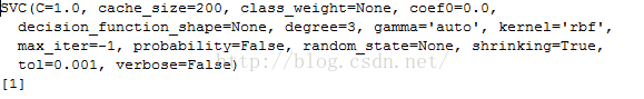
clf = SVC()
clf.fit(X,y)
print clf.fit(X,y)
print clf.predict([[-0.8,-1]])
1
2
3
4
5
6
7
8
9
10
11
12
13
14
15
16
17
18
19
20
21
22
23
24
25
26

• NuSVC（Nu-Support Vector Classification.）：
  核支持向量分类，和SVC类似，也是基于libsvm实现的，但不同的是通过一个参数空值支持向量的个数

示例代码：

NuSVC参数
nu：训练误差的一个上界和支持向量的分数的下界。应在间隔（0，1 ]。
其余同SVC
'''
import numpy as np
X = np.array([[-1, -1], [-2, -1], [1, 1], [2, 1]])
y = np.array([1, 1, 2, 2])
from sklearn.svm import NuSVC
clf = NuSVC()
clf.fit(X, y) 
print clf.fit(X,y)
print(clf.predict([[-0.8, -1]]))
1
2
3
4
5
6
7
8
9
10
11
12

• LinearSVC（Linear Support Vector Classification）：
  线性支持向量分类，类似于SVC，但是其使用的核函数是”linear“上边介绍的两种是按照brf（径向基函数计算的，其实现也不是基于LIBSVM，所以它具有更大的灵活性在选择处罚和损失函数时，而且可以适应更大的数据集，他支持密集和稀疏的输入是通过一对一的方式解决的

LinearSVC 参数解释
C：目标函数的惩罚系数C，用来平衡分类间隔margin和错分样本的，default C = 1.0；
loss ：指定损失函数
penalty ：
dual ：选择算法来解决对偶或原始优化问题。当n_samples > n_features 时dual=false。
tol ：（default = 1e - 3）: svm结束标准的精度;
multi_class：如果y输出类别包含多类，用来确定多类策略， ovr表示一对多，“crammer_singer”优化所有类别的一个共同的目标
如果选择“crammer_singer”，损失、惩罚和优化将会被被忽略。
fit_intercept ：
intercept_scaling ：
class_weight ：对于每一个类别i设置惩罚系数C = class_weight[i]*C,如果不给出，权重自动调整为 n_samples / (n_classes * np.bincount(y))
verbose：跟多线程有关，不大明白啥意思具体
 
from sklearn.svm import LinearSVC
 
X=[[0],[1],[2],[3]]
Y = [0,1,2,3]
 
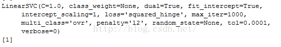
clf = LinearSVC(decision_function_shape='ovo') #ovo为一对一
clf.fit(X,Y)
print clf.fit(X,Y)
 
dec = clf.decision_function([[1]])    #返回的是样本距离超平面的距离
print dec
 
clf.decision_function_shape = "ovr"
dec =clf.decision_function([1]) #返回的是样本距离超平面的距离
print dec
 
#预测
print clf.predict([1])</span>
1
2
3
4
5
6
7
8
9
10
11
12
13
14
15
16
17
18
19
20
21
22
23
24
25
26
27
28
29
30
31

1.Example: Face Recognition（图片多分类）

1.1 查看数据

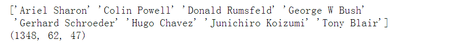
from sklearn.datasets import fetch_lfw_people
faces = fetch_lfw_people(min_faces_per_person=60)
print(faces.target_names)
print(faces.images.shape)
1
2
3
4

1.2 查看前15张图片

fig, ax = plt.subplots(3, 5)
for i, axi in enumerate(ax.flat):
    axi.imshow(faces.images[i], cmap='bone')
    axi.set(xticks=[], yticks=[],
    xlabel=faces.target_names[faces.target[i]])
1
2
3
4
5

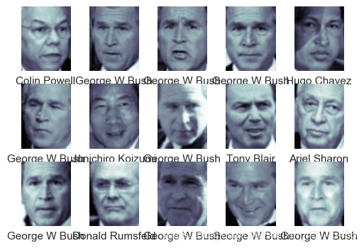
每个图的大小是 [62×47]
在这里我们就把每一个像素点当成了一个特征，但是这样特征太多了，需要用PCA降维一下

1.3 PCA降维与SVM模型的构建

from sklearn.svm import SVC
#from sklearn.decomposition import RandomizedPCA
from sklearn.decomposition import PCA
from sklearn.pipeline import make_pipeline

pca = PCA(n_components=150, whiten=True, random_state=42)#保留150个特征
svc = SVC(kernel='rbf', class_weight='balanced')
model = make_pipeline(pca, svc)
1
2
3
4
5
6
7
8

1.4 划分数据集

from sklearn.model_selection import train_test_split
Xtrain, Xtest, ytrain, ytest = train_test_split(faces.data, faces.target,random_state=40)
1
2

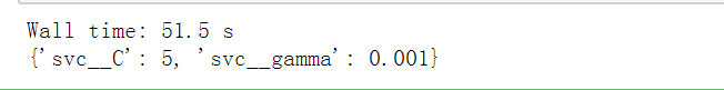
1.5 寻找SVM最优参数（svc__C，svc__gamma）

from sklearn.model_selection import GridSearchCV
param_grid = {'svc__C': [1, 5, 10],
              'svc__gamma': [0.0001, 0.0005, 0.001]}
grid = GridSearchCV(model, param_grid)

%time grid.fit(Xtrain, ytrain)
print(grid.best_params_)
1
2
3
4
5
6
7

1.6 预测结果

model = grid.best_estimator_
yfit = model.predict(Xtest)
yfit.shape
1
2
3

fig, ax = plt.subplots(4, 6)
for i, axi in enumerate(ax.flat):
    axi.imshow(Xtest[i].reshape(62, 47), cmap='bone')
    axi.set(xticks=[], yticks=[])
    axi.set_ylabel(faces.target_names[yfit[i]].split()[-1],
                   color='black' if yfit[i] == ytest[i] else 'red')
fig.suptitle('Predicted Names; Incorrect Labels in Red', size=14);
1
2
3
4
5
6
7

图片标签红色则为分类出错

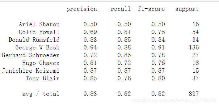
1.7 预测结果评估

from sklearn.metrics import classification_report
print(classification_report(ytest, yfit, target_names=faces.target_names))
1
2

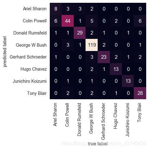
1.8 预测的混淆矩阵

混淆矩阵显示出来能帮助我们查看哪些人更容易弄混

• 精度(precision) = 正确预测的个数(TP)/被预测正确的个数(TP+FP)
• 召回率(recall)=正确预测的个数(TP)/预测个数(TP+FN)
• F1 = 2精度召回率/(精度+召回率)

from sklearn.metrics import confusion_matrix
mat = confusion_matrix(ytest, yfit)
sns.heatmap(mat.T, square=True, annot=True, fmt='d', cbar=False,
            xticklabels=faces.target_names,
            yticklabels=faces.target_names)
plt.xlabel('true label')
plt.ylabel('predicted label');
1
2
3
4
5
6
7

对角线为预测为自己的的正确的个数，非对角线为预测为别人的个数。