

Pandas项目实战1——好莱坞百万级电影评论数据分析
发布于2019-08-20 18:41 阅读(695) 评论(0) 点赞(15) 收藏(2)
好莱坞百万级电影评论数据分析
经过Pandas的入门学习,急需要通过一些简单的项目来将所学知识和用法融会贯通,这里选择对好莱坞百万级电影评论数据进行分析处理,下面就开始吧~
Pandas 知识点
- 数据读取
- 数据集成
- 透视表
- 数据聚合与分组运算
- 分段统计
- 数据可视化
任务需求
- 数据加载和集成
- 平均分较高电影
- 不同性别对电影平均评分
- 不同性别争议最大电影
- 评分次数最多热门的电影
- 不同年龄段争议最大的电影
- 优化与总结
本文所使用的所有数据链接:
链接: https://pan.baidu.com/s/1KBphl8o-YEFXVp8N1IlsgA 提取码: 8daa
操作环境:Jupyter Notebook
1.导入所需库
import numpy as np
import pandas as pd
# draw
import matplotlib.pyplot as plt
%matplotlib inline
- 1
- 2
- 3
- 4
- 5
2.导入数据
读取user
通过查看README可以得到USER数据的格式如下:
USERS FILE DESCRIPTION User information is in the file “users.dat” and is in the following format:
UserID::Gender::Age::Occupation::Zip-code
此处索引命名不一定非要一致,自己明白即可
# shift + Tab 查看函数提示
# 创建索引列表
labels = ['UserID','Gender','Age','Occupation','Zip-code']
# 以此输入路径,分隔符,不作为头部,赋值索引
users = pd.read_csv('./users.dat',sep = '::', header= None, names =labels)
# 读取后查看维度
users.shape
- 1
- 2
- 3
- 4
- 5
- 6
- 7
(6040, 5)
- 1
若有红色输出则即可当做log日志,不用惊慌
users.head()
- 1
| UserID | Gender | Age | Occupation | Zip-code | |
|---|---|---|---|---|---|
| 0 | 1 | F | 1 | 10 | 48067 |
| 1 | 2 | M | 56 | 16 | 70072 |
| 2 | 3 | M | 25 | 15 | 55117 |
| 3 | 4 | M | 45 | 7 | 02460 |
| 4 | 5 | M | 25 | 20 | 55455 |
读取Movie
MOVIES FILE DESCRIPTION
Movie information is in the file “movies.dat” and is in the following
format:MovieID::Title::Genres
labels2 = ['MovieID','Title','Genres']
movie =pd.read_csv('./movies.dat',sep='::',header = None,names=labels2)
# display同时显示两个
display(movie.head(),movie.shape)
- 1
- 2
- 3
- 4
| MovieID | Title | Genres | |
|---|---|---|---|
| 0 | 1 | Toy Story (1995) | Animation|Children’s|Comedy |
| 1 | 2 | Jumanji (1995) | Adventure|Children’s|Fantasy |
| 2 | 3 | Grumpier Old Men (1995) | Comedy|Romance |
| 3 | 4 | Waiting to Exhale (1995) | Comedy|Drama |
| 4 | 5 | Father of the Bride Part II (1995) | Comedy |
(3883, 3)
- 1
读取RATINGS
RATINGS FILE DESCRIPTION
All ratings are contained in the file “ratings.dat” and are in the
following format:UserID::MovieID::Rating::Timestamp
labels3 = ['UserID','MovieID','Rating','Time']
ratings =pd.read_csv('./ratings.dat',sep='::',header = None,names=labels3)
# display()同时显示两组数据
display(ratings.head(),ratings.shape)
- 1
- 2
- 3
- 4
这里读取百万级数据可能需要稍作等待。。。
| UserID | MovieID | Rating | Time | |
|---|---|---|---|---|
| 0 | 1 | 1193 | 5 | 978300760 |
| 1 | 1 | 661 | 3 | 978302109 |
| 2 | 1 | 914 | 3 | 978301968 |
| 3 | 1 | 3408 | 4 | 978300275 |
| 4 | 1 | 2355 | 5 | 978824291 |
(1000209, 4)
- 1
3. 数据合并
由于数据分布在三个表,所以需要对数据进行数据集成,首先将三张表简单展示在一起,查看各自特征。
display(users.head(),movie.head(),ratings.head())
| UserID | Gender | Age | Occupation | Zip-code | |
|---|---|---|---|---|---|
| 0 | 1 | F | 1 | 10 | 48067 |
| 1 | 2 | M | 56 | 16 | 70072 |
| 2 | 3 | M | 25 | 15 | 55117 |
| 3 | 4 | M | 45 | 7 | 02460 |
| 4 | 5 | M | 25 | 20 | 55455 |
| MovieID | Title | Genres | |
|---|---|---|---|
| 0 | 1 | Toy Story (1995) | Animation|Children’s|Comedy |
| 1 | 2 | Jumanji (1995) | Adventure|Children’s|Fantasy |
| 2 | 3 | Grumpier Old Men (1995) | Comedy|Romance |
| 3 | 4 | Waiting to Exhale (1995) | Comedy|Drama |
| 4 | 5 | Father of the Bride Part II (1995) | Comedy |
| UserID | MovieID | Rating | Time | |
|---|---|---|---|---|
| 0 | 1 | 1193 | 5 | 978300760 |
| 1 | 1 | 661 | 3 | 978302109 |
| 2 | 1 | 914 | 3 | 978301968 |
| 3 | 1 | 3408 | 4 | 978300275 |
| 4 | 1 | 2355 | 5 | 978824291 |
经过观察发现后两张表关于MovieID有重合,可以进行数据合并
# 关于MovieID可以合并
df1 = pd.merge(left = movie ,right=ratings)
df1.head(10)
- 1
- 2
- 3
| MovieID | Title | Genres | UserID | Rating | Time | |
|---|---|---|---|---|---|---|
| 0 | 1 | Toy Story (1995) | Animation|Children’s|Comedy | 1 | 5 | 978824268 |
| 1 | 1 | Toy Story (1995) | Animation|Children’s|Comedy | 6 | 4 | 978237008 |
| 2 | 1 | Toy Story (1995) | Animation|Children’s|Comedy | 8 | 4 | 978233496 |
| 3 | 1 | Toy Story (1995) | Animation|Children’s|Comedy | 9 | 5 | 978225952 |
| 4 | 1 | Toy Story (1995) | Animation|Children’s|Comedy | 10 | 5 | 978226474 |
| 5 | 1 | Toy Story (1995) | Animation|Children’s|Comedy | 18 | 4 | 978154768 |
| 6 | 1 | Toy Story (1995) | Animation|Children’s|Comedy | 19 | 5 | 978555994 |
| 7 | 1 | Toy Story (1995) | Animation|Children’s|Comedy | 21 | 3 | 978139347 |
| 8 | 1 | Toy Story (1995) | Animation|Children’s|Comedy | 23 | 4 | 978463614 |
| 9 | 1 | Toy Story (1995) | Animation|Children’s|Comedy | 26 | 3 | 978130703 |
merge()在并没有指定在哪一列进行连接时,连接键信息没有确定,此时merge()会自动将表中重叠列名作为连接的键,但是一般显式的设定链接键是好的习惯。
另外在合并后有可能出现缺少数据的情况,这是因为默认是内连接方式,即为两张表的交集部分进行合并,若是外连接方式则是键的并集,所以在数据合并后检查数据总量是好的习惯。
movie_data = pd.merge(df1,users,how="outer")
movie_data.shape
#检查数据没少
- 1
- 2
- 3
(1000209, 10)
- 1
movie_data.head(10)
| MovieID | Title | Genres | UserID | Rating | Time | Gender | Age | Occupation | Zip-code | |
|---|---|---|---|---|---|---|---|---|---|---|
| 0 | 1 | Toy Story (1995) | Animation|Children’s|Comedy | 1 | 5 | 978824268 | F | 1 | 10 | 48067 |
| 1 | 48 | Pocahontas (1995) | Animation|Children’s|Musical|Romance | 1 | 5 | 978824351 | F | 1 | 10 | 48067 |
| 2 | 150 | Apollo 13 (1995) | Drama | 1 | 5 | 978301777 | F | 1 | 10 | 48067 |
| 3 | 260 | Star Wars: Episode IV - A New Hope (1977) | Action|Adventure|Fantasy|Sci-Fi | 1 | 4 | 978300760 | F | 1 | 10 | 48067 |
| 4 | 527 | Schindler’s List (1993) | Drama|War | 1 | 5 | 978824195 | F | 1 | 10 | 48067 |
| 5 | 531 | Secret Garden, The (1993) | Children’s|Drama | 1 | 4 | 978302149 | F | 1 | 10 | 48067 |
| 6 | 588 | Aladdin (1992) | Animation|Children’s|Comedy|Musical | 1 | 4 | 978824268 | F | 1 | 10 | 48067 |
| 7 | 594 | Snow White and the Seven Dwarfs (1937) | Animation|Children’s|Musical | 1 | 4 | 978302268 | F | 1 | 10 | 48067 |
| 8 | 595 | Beauty and the Beast (1991) | Animation|Children’s|Musical | 1 | 5 | 978824268 | F | 1 | 10 | 48067 |
| 9 | 608 | Fargo (1996) | Crime|Drama|Thriller | 1 | 4 | 978301398 | F | 1 | 10 | 48067 |
# 通过标题查看有多少部电影
movie_data['Title'].unique().size
- 1
- 2
3706
- 1
4.平均分较高电影
既要显示电影名称又要有分数 考虑作透视表
以名称为索引 以分数 并且计算平均分为数值来作透视表
movie_rate_mean = pd.pivot_table(movie_data,values=['Rating'],index=['Title'],aggfunc='mean')
movie_rate_mean.head()
- 1
- 2
| Rating | |
|---|---|
| Title | |
| $1,000,000 Duck (1971) | 3.027027 |
| 'Night Mother (1986) | 3.371429 |
| 'Til There Was You (1997) | 2.692308 |
| 'burbs, The (1989) | 2.910891 |
| …And Justice for All (1979) | 3.713568 |
按照分数排个序 inplace = True 节省内存不会打印输出 直接在原数据进行排序
movie_rate_mean.sort_values(by='Rating',ascending = False,inplace = True)
movie_rate_mean.head(20)
- 1
- 2
| Rating | |
|---|---|
| Title | |
| Ulysses (Ulisse) (1954) | 5.000000 |
| Lured (1947) | 5.000000 |
| Follow the Bitch (1998) | 5.000000 |
| Bittersweet Motel (2000) | 5.000000 |
| Song of Freedom (1936) | 5.000000 |
| One Little Indian (1973) | 5.000000 |
| Smashing Time (1967) | 5.000000 |
| Schlafes Bruder (Brother of Sleep) (1995) | 5.000000 |
| Gate of Heavenly Peace, The (1995) | 5.000000 |
| Baby, The (1973) | 5.000000 |
| I Am Cuba (Soy Cuba/Ya Kuba) (1964) | 4.800000 |
| Lamerica (1994) | 4.750000 |
| Apple, The (Sib) (1998) | 4.666667 |
| Sanjuro (1962) | 4.608696 |
| Seven Samurai (The Magnificent Seven) (Shichinin no samurai) (1954) | 4.560510 |
| Shawshank Redemption, The (1994) | 4.554558 |
| Godfather, The (1972) | 4.524966 |
| Close Shave, A (1995) | 4.520548 |
| Usual Suspects, The (1995) | 4.517106 |
| Schindler’s List (1993) | 4.510417 |
# 查看评分最低的电影 倒序查看
movie_rate_mean[-20:]
- 1
- 2
| Rating | |
|---|---|
| Title | |
| Lotto Land (1995) | 1.0 |
| Nueba Yol (1995) | 1.0 |
| Even Dwarfs Started Small (Auch Zwerge haben klein angefangen) (1971) | 1.0 |
| Get Over It (1996) | 1.0 |
| Venice/Venice (1992) | 1.0 |
| Sleepover (1995) | 1.0 |
| Silence of the Palace, The (Saimt el Qusur) (1994) | 1.0 |
| Waltzes from Vienna (1933) | 1.0 |
| Wirey Spindell (1999) | 1.0 |
| Kestrel’s Eye (Falkens 鰃a) (1998) | 1.0 |
| Spring Fever USA (a.k.a. Lauderdale) (1989) | 1.0 |
| Loves of Carmen, The (1948) | 1.0 |
| Underworld (1997) | 1.0 |
| Low Life, The (1994) | 1.0 |
| Santa with Muscles (1996) | 1.0 |
| Fantastic Night, The (La Nuit Fantastique) (1949) | 1.0 |
| Cheetah (1989) | 1.0 |
| Torso (Corpi Presentano Tracce di Violenza Carnale) (1973) | 1.0 |
| Mutters Courage (1995) | 1.0 |
| Windows (1980) | 1.0 |
5. 不同性别对电影评分
依然是通过性别索引来建立透视表分析数据
movie_gender_rating = pd.pivot_table(movie_data,values=['Rating'],index=['Title','Gender'],aggfunc='mean')
movie_gender_rating.head(10)
- 1
- 2
| Rating | ||
|---|---|---|
| Title | Gender | |
| $1,000,000 Duck (1971) | F | 3.375000 |
| M | 2.761905 | |
| 'Night Mother (1986) | F | 3.388889 |
| M | 3.352941 | |
| 'Til There Was You (1997) | F | 2.675676 |
| M | 2.733333 | |
| 'burbs, The (1989) | F | 2.793478 |
| M | 2.962085 | |
| …And Justice for All (1979) | F | 3.828571 |
| M | 3.689024 |
这样分析数据似乎不是非常直观,且由于只分析分值所以可以不显示Rating数据
# 换种透视方法 去掉values中括号->去掉rating标题
movie_gender_rating2 = pd.pivot_table(movie_data,values='Rating',index=['Title'],columns=['Gender'],aggfunc='mean')
movie_gender_rating2.head()
- 1
- 2
- 3
| Gender | F | M |
|---|---|---|
| Title | ||
| $1,000,000 Duck (1971) | 3.375000 | 2.761905 |
| 'Night Mother (1986) | 3.388889 | 3.352941 |
| 'Til There Was You (1997) | 2.675676 | 2.733333 |
| 'burbs, The (1989) | 2.793478 | 2.962085 |
| …And Justice for All (1979) | 3.828571 | 3.689024 |
6.不同性别争议最大的电影
查看列索引
movie_gender_rating2.columns
- 1
Index(['F', 'M'], dtype='object', name='Gender')
- 1
创建新的列diff用来存放男女评分差异
#男女评分差异
movie_gender_rating2['diff'] = movie_gender_rating2.F - movie_gender_rating2.M
movie_gender_rating2.head()
- 1
- 2
- 3
| Gender | F | M | diff |
|---|---|---|---|
| Title | |||
| $1,000,000 Duck (1971) | 3.375000 | 2.761905 | 0.613095 |
| 'Night Mother (1986) | 3.388889 | 3.352941 | 0.035948 |
| 'Til There Was You (1997) | 2.675676 | 2.733333 | -0.057658 |
| 'burbs, The (1989) | 2.793478 | 2.962085 | -0.168607 |
| …And Justice for All (1979) | 3.828571 | 3.689024 | 0.139547 |
要分析差异最大,可以对数据进行正向排序
movie_gender_rating2.sort_values(by="diff",ascending=False,inplace=True)
movie_gender_rating2.head()
- 1
- 2
| Gender | F | M | diff |
|---|---|---|---|
| Title | |||
| James Dean Story, The (1957) | 4.000000 | 1.000000 | 3.000000 |
| Spiders, The (Die Spinnen, 1. Teil: Der Goldene See) (1919) | 4.000000 | 1.000000 | 3.000000 |
| Country Life (1994) | 5.000000 | 2.000000 | 3.000000 |
| Babyfever (1994) | 3.666667 | 1.000000 | 2.666667 |
| Woman of Paris, A (1923) | 5.000000 | 2.428571 | 2.571429 |
因为是女减去男 所以差异最大的,是女性最喜欢的
f = movie_gender_rating2[:10]
f
- 1
- 2
| Gender | F | M | diff |
|---|---|---|---|
| Title | |||
| James Dean Story, The (1957) | 4.000000 | 1.000000 | 3.000000 |
| Spiders, The (Die Spinnen, 1. Teil: Der Goldene See) (1919) | 4.000000 | 1.000000 | 3.000000 |
| Country Life (1994) | 5.000000 | 2.000000 | 3.000000 |
| Babyfever (1994) | 3.666667 | 1.000000 | 2.666667 |
| Woman of Paris, A (1923) | 5.000000 | 2.428571 | 2.571429 |
| Cobra (1925) | 4.000000 | 1.500000 | 2.500000 |
| Other Side of Sunday, The (S鴑dagsengler) (1996) | 5.000000 | 2.928571 | 2.071429 |
| Theodore Rex (1995) | 3.000000 | 1.000000 | 2.000000 |
| For the Moment (1994) | 5.000000 | 3.000000 | 2.000000 |
| Separation, The (La S閜aration) (1994) | 4.000000 | 2.000000 | 2.000000 |
此时排在最后的就是男减女差异最大的也就是男性最喜欢的
# 最后十个就男性最喜欢的
m = movie_gender_rating2[-10:]
#处理一下 去掉存在的许多NAN
m = movie_gender_rating2.dropna()[-10:]
m
- 1
- 2
- 3
- 4
- 5
| Gender | F | M | diff |
|---|---|---|---|
| Title | |||
| Jamaica Inn (1939) | 1.0 | 3.142857 | -2.142857 |
| Flying Saucer, The (1950) | 1.0 | 3.300000 | -2.300000 |
| Rosie (1998) | 1.0 | 3.333333 | -2.333333 |
| In God’s Hands (1998) | 1.0 | 3.333333 | -2.333333 |
| Dangerous Ground (1997) | 1.0 | 3.333333 | -2.333333 |
| Killer: A Journal of Murder (1995) | 1.0 | 3.428571 | -2.428571 |
| Stalingrad (1993) | 1.0 | 3.593750 | -2.593750 |
| Enfer, L’ (1994) | 1.0 | 3.750000 | -2.750000 |
| Neon Bible, The (1995) | 1.0 | 4.000000 | -3.000000 |
| Tigrero: A Film That Was Never Made (1994) | 1.0 | 4.333333 | -3.333333 |
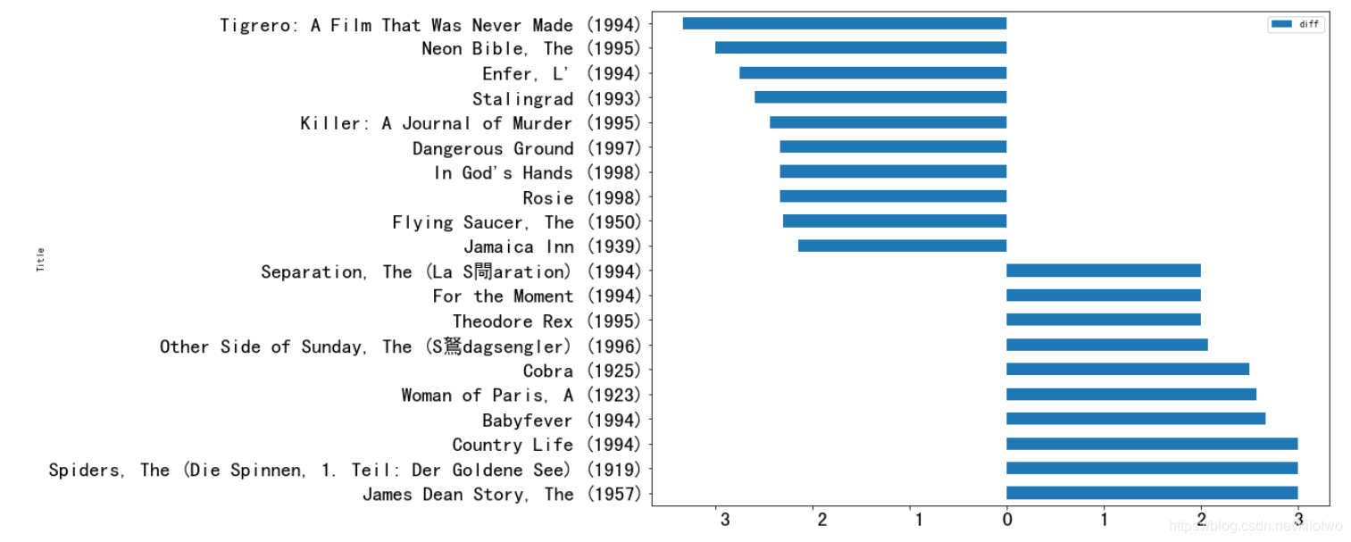
将男女最喜欢的电影合并成一张表,便于作图观察
diff = pd.concat([f,m])
diff
- 1
- 2
| Gender | F | M | diff |
|---|---|---|---|
| Title | |||
| James Dean Story, The (1957) | 4.000000 | 1.000000 | 3.000000 |
| Spiders, The (Die Spinnen, 1. Teil: Der Goldene See) (1919) | 4.000000 | 1.000000 | 3.000000 |
| Country Life (1994) | 5.000000 | 2.000000 | 3.000000 |
| Babyfever (1994) | 3.666667 | 1.000000 | 2.666667 |
| Woman of Paris, A (1923) | 5.000000 | 2.428571 | 2.571429 |
| Cobra (1925) | 4.000000 | 1.500000 | 2.500000 |
| Other Side of Sunday, The (S鴑dagsengler) (1996) | 5.000000 | 2.928571 | 2.071429 |
| Theodore Rex (1995) | 3.000000 | 1.000000 | 2.000000 |
| For the Moment (1994) | 5.000000 | 3.000000 | 2.000000 |
| Separation, The (La S閜aration) (1994) | 4.000000 | 2.000000 | 2.000000 |
| Jamaica Inn (1939) | 1.000000 | 3.142857 | -2.142857 |
| Flying Saucer, The (1950) | 1.000000 | 3.300000 | -2.300000 |
| Rosie (1998) | 1.000000 | 3.333333 | -2.333333 |
| In God’s Hands (1998) | 1.000000 | 3.333333 | -2.333333 |
| Dangerous Ground (1997) | 1.000000 | 3.333333 | -2.333333 |
| Killer: A Journal of Murder (1995) | 1.000000 | 3.428571 | -2.428571 |
| Stalingrad (1993) | 1.000000 | 3.593750 | -2.593750 |
| Enfer, L’ (1994) | 1.000000 | 3.750000 | -2.750000 |
| Neon Bible, The (1995) | 1.000000 | 4.000000 | -3.000000 |
| Tigrero: A Film That Was Never Made (1994) | 1.000000 | 4.333333 | -3.333333 |
分析结果 进行数据可视化
# barh水平柱状图
diff.plot(y='diff',kind='barh',figsize=(16,9))
- 1
- 2
7.评论次数最多热门的电影
次数最多考虑利用groupby按照title来做电影的数据聚合,采用size得出每种电影的次数进行排序
# 用groupby 按照title 来做数据聚合
rating_count = movie_data.groupby(['Title']).size()
rating_count.sort_values(ascending = False)
- 1
- 2
- 3
Title
American Beauty (1999)                                   3428
Star Wars: Episode IV - A New Hope (1977)                2991
Star Wars: Episode V - The Empire Strikes Back (1980)    2990
Star Wars: Episode VI - Return of the Jedi (1983)        2883
Jurassic Park (1993)                                     2672
- 1
- 2
- 3
- 4
- 5
- 6
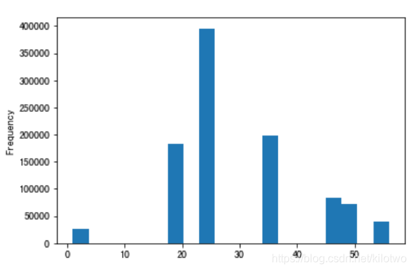
8.查看不同年龄段争议最大电影
分析不同年龄段需要对用户的年龄分布图作图分析
movie_data['Age'].plot(kind = 'hist',bins = 20)
- 1
用pandas.cut 函数将用户年龄分组
# 建立分组索引
labels4 = ['0-9','10-19','20-29','30-39','40-49','50-59']
# range是左闭右开 所以取到61
movie_data['Age_range']=pd.cut(movie_data.Age,bins=range(0,61,10),labels=labels4)
movie_data.head()
- 1
- 2
- 3
- 4
- 5
| MovieID | Title | Genres | UserID | Rating | Time | Gender | Age | Occupation | Zip-code | Age_range | |
|---|---|---|---|---|---|---|---|---|---|---|---|
| 0 | 1 | Toy Story (1995) | Animation|Children’s|Comedy | 1 | 5 | 978824268 | F | 1 | 10 | 48067 | 0-9 |
| 1 | 48 | Pocahontas (1995) | Animation|Children’s|Musical|Romance | 1 | 5 | 978824351 | F | 1 | 10 | 48067 | 0-9 |
| 2 | 150 | Apollo 13 (1995) | Drama | 1 | 5 | 978301777 | F | 1 | 10 | 48067 | 0-9 |
| 3 | 260 | Star Wars: Episode IV - A New Hope (1977) | Action|Adventure|Fantasy|Sci-Fi | 1 | 4 | 978300760 | F | 1 | 10 | 48067 | 0-9 |
| 4 | 527 | Schindler’s List (1993) | Drama|War | 1 | 5 | 978824195 | F | 1 | 10 | 48067 | 0-9 |
9.每个年龄段用户评分人数和打分偏好
# agg 用来计算多个数据
movie_data.groupby('Age_range').agg({'Rating':[np.size,np.mean]})
- 1
- 2
| Rating | ||
|---|---|---|
| size | mean | |
| Age_range | ||
| 0-9 | 27211 | 3.549520 |
| 10-19 | 183536 | 3.507573 |
| 20-29 | 395556 | 3.545235 |
| 30-39 | 199003 | 3.618162 |
| 40-49 | 156123 | 3.673559 |
| 50-59 | 38780 | 3.766632 |
10.优化数据分析,结果真实可靠
由于评分次数相差悬殊,导致有的电影评分人数少,却得到很高的分数
解决方案: 加入评分次数考核限制
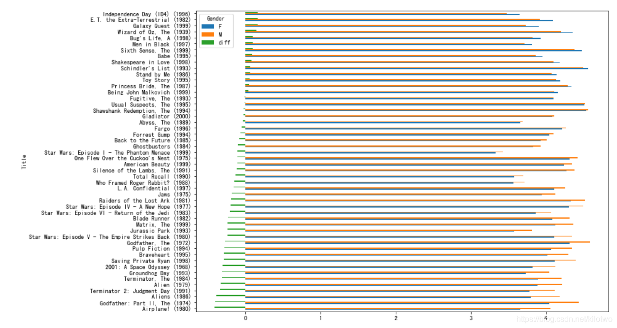
10.1 加入评分次数限制来分析不同性别对电影的平均分
# 评论最多的50部电影排行
top_movie_title = movie_data.groupby('Title').size().sort_values()[::-1][:50].index
top_movie_title
- 1
- 2
- 3
Index(['American Beauty (1999)', 'Star Wars: Episode IV - A New Hope (1977)',
       'Star Wars: Episode V - The Empire Strikes Back (1980)',
       'Star Wars: Episode VI - Return of the Jedi (1983)',
       'Jurassic Park (1993)', 'Saving Private Ryan (1998)',
       'Terminator 2: Judgment Day (1991)', 'Matrix, The (1999)',
       'Back to the Future (1985)', 'Silence of the Lambs, The (1991)',
       'Men in Black (1997)', 'Raiders of the Lost Ark (1981)', 'Fargo (1996)',
       'Sixth Sense, The (1999)', 'Braveheart (1995)',
       'Shakespeare in Love (1998)', 'Princess Bride, The (1987)',
       'Schindler's List (1993)', 'L.A. Confidential (1997)',
       'Groundhog Day (1993)', 'E.T. the Extra-Terrestrial (1982)',
       'Star Wars: Episode I - The Phantom Menace (1999)',
       'Being John Malkovich (1999)', 'Shawshank Redemption, The (1994)',
       'Godfather, The (1972)', 'Forrest Gump (1994)', 'Ghostbusters (1984)',
       'Pulp Fiction (1994)', 'Terminator, The (1984)', 'Toy Story (1995)',
       'Alien (1979)', 'Total Recall (1990)', 'Fugitive, The (1993)',
       'Gladiator (2000)', 'Aliens (1986)', 'Blade Runner (1982)',
       'Who Framed Roger Rabbit? (1988)', 'Stand by Me (1986)',
       'Usual Suspects, The (1995)', 'Babe (1995)', 'Airplane! (1980)',
       'Independence Day (ID4) (1996)', 'Galaxy Quest (1999)',
       'One Flew Over the Cuckoo's Nest (1975)', 'Wizard of Oz, The (1939)',
       '2001: A Space Odyssey (1968)', 'Abyss, The (1989)',
       'Bug's Life, A (1998)', 'Jaws (1975)',
       'Godfather: Part II, The (1974)'],
      dtype='object', name='Title')
- 1
- 2
- 3
- 4
- 5
- 6
- 7
- 8
- 9
- 10
- 11
- 12
- 13
- 14
- 15
- 16
- 17
- 18
- 19
- 20
- 21
- 22
- 23
- 24
- 25
这里需要得到这50部电影的布尔索引,用来刷选男女差异最大的电影
# 获取布尔索引
flag = movie_gender_rating2.index.isin(top_movie_title)
flag
- 1
- 2
- 3
df1 = movie_gender_rating2[flag].sort_values(by='diff')
df1.plot(kind ='barh',figsize =(12,9))
- 1
- 2
10.2 加入评分次数限制分析平均分高的电影
movie_rating_mean = pd.pivot_table(movie_data,values='Rating',index='Title')
# 这里依然首先获取最受欢迎布尔索引
index = movie_data.groupby('Title').size().sort_values()[::-1][:50].index
flag2 = movie_rating_mean.index.isin(index)
# 利用布尔索引筛选平均分数组中最受欢迎的电影
movie_rating_top_mean = movie_rating_mean[flag2]
# 进行排序
movie_rating_top_mean.sort_values(by='Rating',ascending = False).head(10)
- 1
- 2
- 3
- 4
- 5
- 6
- 7
- 8
| Rating | |
|---|---|
| Title | |
| Shawshank Redemption, The (1994) | 4.554558 |
| Godfather, The (1972) | 4.524966 |
| Usual Suspects, The (1995) | 4.517106 |
| Schindler’s List (1993) | 4.510417 |
| Raiders of the Lost Ark (1981) | 4.477725 |
| Star Wars: Episode IV - A New Hope (1977) | 4.453694 |
| Sixth Sense, The (1999) | 4.406263 |
| One Flew Over the Cuckoo’s Nest (1975) | 4.390725 |
| Godfather: Part II, The (1974) | 4.357565 |
| Silence of the Lambs, The (1991) | 4.351823 |
总结
在数据处理过程中,合并、透视、分组、排序最为常用,通过此项目,熟悉了Pandas在处理百万级数据时的基本操作和一些常用API调用方法,了解到数据分析处理工作的流程,为后续深入学习打下基础。
所属网站分类: 技术文章 > 博客
作者:j878
链接:https://www.pythonheidong.com/blog/article/49541/64abda19986e7b161b06/
来源:python黑洞网
任何形式的转载都请注明出处,如有侵权 一经发现 必将追究其法律责任
昵称:
评论内容:(最多支持255个字符)
---无人问津也好,技不如人也罢,你都要试着安静下来,去做自己该做的事,而不是让内心的烦躁、焦虑,坏掉你本来就不多的热情和定力