引言

TensorFlow 是一个采用数据流图，用于数值计算的开源软件库。它是一个不严格的“神经网络”库，可以利用它提供的模块搭建大多数类型的神经网络。它可以基于ＣＰＵ或ＧＰＵ运行，可以自动使用ＧＰＵ，无需编写分配程序，主要支持Python编写。
MNIST 是一个巨大的手写数字数据集，被广泛应用于机器学习识别领域。MNIST有60000张训练集数据和10000张测试集数据，每一个训练元素都是28*28像素的手写数字图片。作为一个常见的数据集，MNIST经常被用来测试神经网络，也是比较基本的应用。官网下载地址：http://yann.lecun.com/exdb/mnist/。

关于TensorFlow的安装

CPU版： 在cmd命令行中输入pip install tensorflow即可。这边建议不用安装太新的版本，1.11.0版本就足够用了，版本太新反而可能出现错误。CPU版安装虽然简单，但是对于训练数据集巨大的工程运行起来效率却不是很高（当然电脑配置好的可以忽略这条。）
GPU版： （在确保自己电脑有英伟达显卡的情况下，没有的话只能安装CPU版） GPU版的也要在命令行下先安装TensorFlow，输入pip install tensorflow-gpu即可安装。然后再安装CUDA CUDNN这两个软件，注意版本相对应！不然会报错。 下图为其之间的对应版本。这边推荐装CUDA 9.0的。GPU版本安装相对复杂，但运行速度会比CPU版本快。

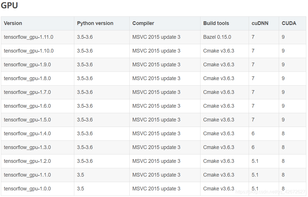
至于具体的安装步骤，可以参考这篇博客TensorFlow GPU版详细安装步骤，这边就不细说。

CNN算法

对于识别算法主要使用的是卷积神经网络算法（CNN）

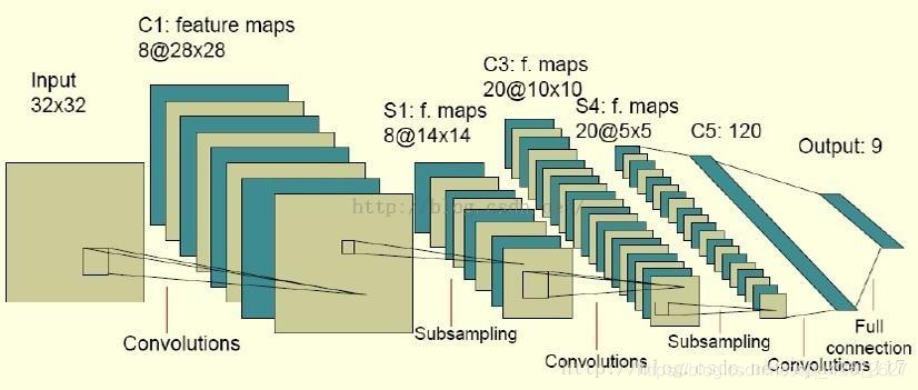
主要结构为：输入-卷积层-池化层-卷积层-池化层-全连接层-输出。
卷积： 卷积其实可以看做是提取特征的过程。通过卷积提取特征值来简化输入。如果不使用卷积的话，整个网络的输入量就是整张图片，处理就很困难。
池化： 池化是用来把卷积结果进行压缩，进一步减少全连接时的连接数。 池化有两种：
一种是最大池化，在选中区域中找最大的值作为抽样后的值； 一种是平均值池化，把选中的区域中的平均值作为抽样后的值。
全连接： 把分布式特征representation映射到样本标记空间，简言之就是特征分类。

代码

1.trainMnistFromPackage

import tensorflow as tf
import numpy as np # 习惯加上这句，但这边没有用到
from tensorflow.examples.tutorials.mnist import input_data
import matplotlib.pyplot as plt
mnist = input_data.read_data_sets('MNIST_data/', one_hot=True)

sess = tf.InteractiveSession()

# 1、权重初始化,偏置初始化
# 为了创建这个模型，我们需要创建大量的权重和偏置项
# 为了不在建立模型的时候反复操作，定义两个函数用于初始化
def weight_variable(shape):
    initial = tf.truncated_normal(shape,stddev=0.1)#正太分布的标准差设为0.1
    return tf.Variable(initial)
def bias_variable(shape):
    initial = tf.constant(0.1,shape=shape)
    return tf.Variable(initial)


# 2、卷积层和池化层也是接下来要重复使用的，因此也为它们定义创建函数
# tf.nn.conv2d是Tensorflow中的二维卷积函数，参数x是输入，w是卷积的参数
# strides代表卷积模块移动的步长，都是1代表会不遗漏地划过图片的每一个点，padding代表边界的处理方式
# padding = 'SAME'，表示padding后卷积的图与原图尺寸一致，激活函数relu()
# tf.nn.max_pool是Tensorflow中的最大池化函数，这里使用2 * 2 的最大池化，即将2 * 2 的像素降为1 * 1的像素
# 最大池化会保留原像素块中灰度值最高的那一个像素，即保留最显著的特征，因为希望整体缩小图片尺寸
# ksize：池化窗口的大小，取一个四维向量，一般是[1,height,width,1]
# 因为我们不想再batch和channel上做池化，一般也是[1,stride,stride,1]
def conv2d(x, w):
    return tf.nn.conv2d(x, w, strides=[1,1,1,1],padding='SAME') # 保证输出和输入是同样大小
def max_pool_2x2(x):
    return tf.nn.max_pool(x, ksize=[1,2,2,1], strides=[1,2,2,1],padding='SAME')


# 3、参数
# 这里的x,y_并不是特定的值，它们只是一个占位符，可以在TensorFlow运行某一计算时根据该占位符输入具体的值
# 输入图片x是一个2维的浮点数张量，这里分配给它的shape为[None, 784]，784是一张展平的MNIST图片的维度
# None 表示其值的大小不定，在这里作为第1个维度值，用以指代batch的大小，means x 的数量不定
# 输出类别y_也是一个2维张量，其中每一行为一个10维的one_hot向量，用于代表某一MNIST图片的类别
x = tf.placeholder(tf.float32, [None,784], name="x-input")
y_ = tf.placeholder(tf.float32,[None,10]) # 10列


# 4、第一层卷积，它由一个卷积接一个max pooling完成
# 张量形状[5,5,1,32]代表卷积核尺寸为5 * 5，1个颜色通道，32个通道数目
w_conv1 = weight_variable([5,5,1,32])
b_conv1 = bias_variable([32]) # 每个输出通道都有一个对应的偏置量
# 我们把x变成一个4d 向量其第2、第3维对应图片的宽、高，最后一维代表图片的颜色通道数(灰度图的通道数为1，如果是RGB彩色图，则为3)
x_image = tf.reshape(x,[-1,28,28,1])
# 因为只有一个颜色通道，故最终尺寸为[-1，28，28，1]，前面的-1代表样本数量不固定，最后的1代表颜色通道数量
h_conv1 = tf.nn.relu(conv2d(x_image, w_conv1) + b_conv1) # 使用conv2d函数进行卷积操作，非线性处理
h_pool1 = max_pool_2x2(h_conv1)                          # 对卷积的输出结果进行池化操作


# 5、第二个和第一个一样，是为了构建一个更深的网络，把几个类似的堆叠起来
# 第二层中，每个5 * 5 的卷积核会得到64个特征
w_conv2 = weight_variable([5,5,32,64])
b_conv2 = bias_variable([64])
h_conv2 = tf.nn.relu(conv2d(h_pool1, w_conv2) + b_conv2)# 输入的是第一层池化的结果
h_pool2 = max_pool_2x2(h_conv2)

# 6、密集连接层
# 图片尺寸减小到7 * 7，加入一个有1024个神经元的全连接层，
# 把池化层输出的张量reshape(此函数可以重新调整矩阵的行、列、维数)成一些向量，加上偏置，然后对其使用Relu激活函数
w_fc1 = weight_variable([7 * 7 * 64, 1024])
b_fc1 = bias_variable([1024])
h_pool2_flat = tf.reshape(h_pool2, [-1,7 * 7 * 64])
h_fc1 = tf.nn.relu(tf.matmul(h_pool2_flat, w_fc1) + b_fc1)

# 7、使用dropout，防止过度拟合
# dropout是在神经网络里面使用的方法，以此来防止过拟合
# 用一个placeholder来代表一个神经元的输出
# tf.nn.dropout操作除了可以屏蔽神经元的输出外，
# 还会自动处理神经元输出值的scale，所以用dropout的时候可以不用考虑scale
keep_prob = tf.placeholder(tf.float32, name="keep_prob")# placeholder是占位符
h_fc1_drop = tf.nn.dropout(h_fc1, keep_prob)


# 8、输出层，最后添加一个softmax层
w_fc2 = weight_variable([1024,10])
b_fc2 = bias_variable([10])
y_conv = tf.nn.softmax(tf.matmul(h_fc1_drop, w_fc2) + b_fc2, name="y-pred")


# 9、训练和评估模型
# 损失函数是目标类别和预测类别之间的交叉熵
# 参数keep_prob控制dropout比例，然后每100次迭代输出一次日志
cross_entropy = tf.reduce_sum(-tf.reduce_sum(y_ * tf.log(y_conv),reduction_indices=[1]))
train_step = tf.train.AdamOptimizer(1e-4).minimize(cross_entropy)
# 预测结果与真实值的一致性，这里产生的是一个bool型的向量
correct_prediction = tf.equal(tf.argmax(y_conv, 1), tf.argmax(y_, 1))
# 将bool型转换成float型，然后求平均值，即正确的比例
accuracy = tf.reduce_mean(tf.cast(correct_prediction, tf.float32))
# 初始化所有变量，在2017年3月2号以后,用 tf.global_variables_initializer()替代tf.initialize_all_variables()
sess.run(tf.initialize_all_variables())

# 保存最后一个模型
saver = tf.train.Saver(max_to_keep=1)

for i in range(1000):
    batch = mnist.train.next_batch(64)
    if i % 100 == 0:
        train_accuracy = accuracy.eval(feed_dict={x: batch[0], y_: batch[1],keep_prob: 1.0})
        print("Step %d ,training accuracy %g" % (i, train_accuracy))
    train_step.run(feed_dict={x: batch[0], y_: batch[1], keep_prob: 0.5})
print("test accuracy %f " % accuracy.eval(feed_dict={x: mnist.test.images, y_: mnist.test.labels, keep_prob: 1.0}))

# 保存模型于文件夹
saver.save(sess,"save/model")
1
2
3
4
5
6
7
8
9
10
11
12
13
14
15
16
17
18
19
20
21
22
23
24
25
26
27
28
29
30
31
32
33
34
35
36
37
38
39
40
41
42
43
44
45
46
47
48
49
50
51
52
53
54
55
56
57
58
59
60
61
62
63
64
65
66
67
68
69
70
71
72
73
74
75
76
77
78
79
80
81
82
83
84
85
86
87
88
89
90
91
92
93
94
95
96
97
98
99
100
101
102
103
104
105
106
107
108

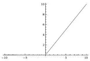
附 RELU激活函数： 小于0的值就变成0，大于0的等于它本身。函数图像如下：

softmax回归： 这是一个分类器，可以认为是Logistic回归的扩展，Logistic大家应该都听说过，就是生物学上的S型曲线，它只能分两类，用0和1表示，这个用来表示答题对错之类只有两种状态的问题时足够了，但是像这里的MNIST要把它分成10类，就必须用softmax来进行分类了。 P(y=0)=p0,P(y=1)=p1,p(y=2)=p2…P(y=9)=p9.这些表示预测为数字i的概率，（跟上面标签的格式正好对应起来了）,它们的和为1，即 ∑(pi)=1。

运行结果

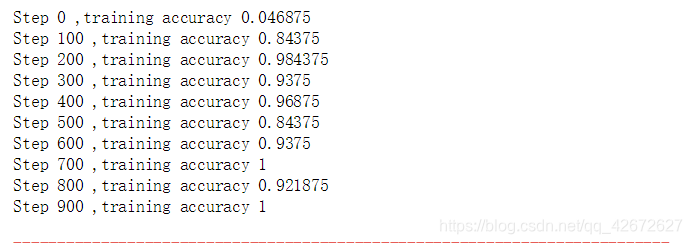
可以看出训练的模型准确率还是可以的。运行过程可能会因为显存不够而报错，需要多运行几次。

2.trainMnistFromImagine

import os 
import cv2 
import numpy as np
import tensorflow as tf
from tensorflow.examples.tutorials.mnist import input_data

sess = tf.InteractiveSession()


def getTrain():
    train=[[],[]] # 指定训练集的格式，一维为输入数据，一维为其标签
    # 读取所有训练图像，作为训练集
    train_root="mnist_train" 
    labels = os.listdir(train_root)
    for label in labels:
        imgpaths = os.listdir(os.path.join(train_root,label))
        for imgname in imgpaths:
            img = cv2.imread(os.path.join(train_root,label,imgname),0)
            array = np.array(img).flatten() # 将二维图像平铺为一维图像
            array=MaxMinNormalization(array)
            train[0].append(array)
            label_ = [0,0,0,0,0,0,0,0,0,0]
            label_[int(label)] = 1
            train[1].append(label_)
    train = shuff(train)
    return train

def getTest():
    test=[[],[]] # 指定训练集的格式，一维为输入数据，一维为其标签
    # 读取所有训练图像，作为训练集
    test_root="mnist_test" 
    labels = os.listdir(test_root)
    for label in labels:
        imgpaths = os.listdir(os.path.join(test_root,label))
        for imgname in imgpaths:
            img = cv2.imread(os.path.join(test_root,label,imgname),0)
            array = np.array(img).flatten() # 将二维图像平铺为一维图像
            array=MaxMinNormalization(array)
            test[0].append(array)
            label_ = [0,0,0,0,0,0,0,0,0,0]
            label_[int(label)] = 1
            test[1].append(label_)
    test = shuff(test)
    return test[0],test[1]

def shuff(data):
    temp=[]
    for i in range(len(data[0])):
        temp.append([data[0][i],data[1][i]])
    import random
    random.shuffle(temp)
    data=[[],[]]
    for tt in temp:
        data[0].append(tt[0])
        data[1].append(tt[1])
    return data

count = 0
def getBatchNum(batch_size,maxNum):
    global count
    if count ==0:
        count=count+batch_size
        return 0,min(batch_size,maxNum)
    else:
        temp = count
        count=count+batch_size
        if min(count,maxNum)==maxNum:
            count=0
            return getBatchNum(batch_size,maxNum)
        return temp,min(count,maxNum)
    
def MaxMinNormalization(x):
    x = (x - np.min(x)) / (np.max(x) - np.min(x))
    return x


# 1、权重初始化,偏置初始化
# 为了创建这个模型，我们需要创建大量的权重和偏置项
# 为了不在建立模型的时候反复操作，定义两个函数用于初始化
def weight_variable(shape):
    initial = tf.truncated_normal(shape,stddev=0.1)#正太分布的标准差设为0.1
    return tf.Variable(initial)
def bias_variable(shape):
    initial = tf.constant(0.1,shape=shape)
    return tf.Variable(initial)


# 2、卷积层和池化层也是接下来要重复使用的，因此也为它们定义创建函数
# tf.nn.conv2d是Tensorflow中的二维卷积函数，参数x是输入，w是卷积的参数
# strides代表卷积模块移动的步长，都是1代表会不遗漏地划过图片的每一个点，padding代表边界的处理方式
# padding = 'SAME'，表示padding后卷积的图与原图尺寸一致，激活函数relu()
# tf.nn.max_pool是Tensorflow中的最大池化函数，这里使用2 * 2 的最大池化，即将2 * 2 的像素降为1 * 1的像素
# 最大池化会保留原像素块中灰度值最高的那一个像素，即保留最显著的特征，因为希望整体缩小图片尺寸
# ksize：池化窗口的大小，取一个四维向量，一般是[1,height,width,1]
# 因为我们不想再batch和channel上做池化，一般也是[1,stride,stride,1]
def conv2d(x, w):
    return tf.nn.conv2d(x, w, strides=[1,1,1,1],padding='SAME') # 保证输出和输入是同样大小
def max_pool_2x2(x):
    return tf.nn.max_pool(x, ksize=[1,2,2,1], strides=[1,2,2,1],padding='SAME')
    
iterNum = 8
batch_size=64 #随机批量下降(64)

print("load train dataset.")
train=getTrain()
print("load test dataset.")
test0,test1=getTest()


# 3、参数
# 这里的x,y_并不是特定的值，它们只是一个占位符，可以在TensorFlow运行某一计算时根据该占位符输入具体的值
# 输入图片x是一个2维的浮点数张量，这里分配给它的shape为[None, 784]，784是一张展平的MNIST图片的维度
# None 表示其值的大小不定，在这里作为第1个维度值，用以指代batch的大小，means x 的数量不定
# 输出类别y_也是一个2维张量，其中每一行为一个10维的one_hot向量，用于代表某一MNIST图片的类别
x = tf.placeholder(tf.float32, [None,784], name="x-input")
y_ = tf.placeholder(tf.float32,[None,10]) # 10列


# 4、第一层卷积，它由一个卷积接一个max pooling完成
# 张量形状[5,5,1,32]代表卷积核尺寸为5 * 5，1个颜色通道，32个通道数目
w_conv1 = weight_variable([5,5,1,32])
b_conv1 = bias_variable([32]) # 每个输出通道都有一个对应的偏置量
# 我们把x变成一个4d 向量其第2、第3维对应图片的宽、高，最后一维代表图片的颜色通道数(灰度图的通道数为1，如果是RGB彩色图，则为3)
x_image = tf.reshape(x,[-1,28,28,1])
# 因为只有一个颜色通道，故最终尺寸为[-1，28，28，1]，前面的-1代表样本数量不固定，最后的1代表颜色通道数量
h_conv1 = tf.nn.relu(conv2d(x_image, w_conv1) + b_conv1) # 使用conv2d函数进行卷积操作，非线性处理
h_pool1 = max_pool_2x2(h_conv1)                          # 对卷积的输出结果进行池化操作


# 5、第二个和第一个一样，是为了构建一个更深的网络，把几个类似的堆叠起来
# 第二层中，每个5 * 5 的卷积核会得到64个特征
w_conv2 = weight_variable([5,5,32,64])
b_conv2 = bias_variable([64])
h_conv2 = tf.nn.relu(conv2d(h_pool1, w_conv2) + b_conv2)# 输入的是第一层池化的结果
h_pool2 = max_pool_2x2(h_conv2)

# 6、密集连接层
# 图片尺寸减小到7 * 7，加入一个有1024个神经元的全连接层，
# 把池化层输出的张量reshape(此函数可以重新调整矩阵的行、列、维数)成一些向量，加上偏置，然后对其使用Relu激活函数
w_fc1 = weight_variable([7 * 7 * 64, 1024])
b_fc1 = bias_variable([1024])
h_pool2_flat = tf.reshape(h_pool2, [-1,7 * 7 * 64])
h_fc1 = tf.nn.relu(tf.matmul(h_pool2_flat, w_fc1) + b_fc1)

# 7、使用dropout，防止过度拟合
# dropout是在神经网络里面使用的方法，以此来防止过拟合
# 用一个placeholder来代表一个神经元的输出
# tf.nn.dropout操作除了可以屏蔽神经元的输出外，
# 还会自动处理神经元输出值的scale，所以用dropout的时候可以不用考虑scale
keep_prob = tf.placeholder(tf.float32, name="keep_prob")# placeholder是占位符
h_fc1_drop = tf.nn.dropout(h_fc1, keep_prob)


# 8、输出层，最后添加一个softmax层
w_fc2 = weight_variable([1024,10])
b_fc2 = bias_variable([10])
y_conv = tf.nn.softmax(tf.matmul(h_fc1_drop, w_fc2) + b_fc2, name="y-pred")


# 9、训练和评估模型
# 损失函数是目标类别和预测类别之间的交叉熵
# 参数keep_prob控制dropout比例，然后每100次迭代输出一次日志
cross_entropy = tf.reduce_sum(-tf.reduce_sum(y_ * tf.log(y_conv),reduction_indices=[1]))
train_step = tf.train.AdamOptimizer(1e-4).minimize(cross_entropy)
# 预测结果与真实值的一致性，这里产生的是一个bool型的向量
correct_prediction = tf.equal(tf.argmax(y_conv, 1), tf.argmax(y_, 1))
# 将bool型转换成float型，然后求平均值，即正确的比例
accuracy = tf.reduce_mean(tf.cast(correct_prediction, tf.float32))
# 初始化所有变量，在2017年3月2号以后,用 tf.global_variables_initializer()替代tf.initialize_all_variables()
sess.run(tf.initialize_all_variables())

# 保存最后一个模型
saver = tf.train.Saver(max_to_keep=1)


for i in range(iterNum):
    for j in range(int(len(train[1])/batch_size)):
        imagesNum=getBatchNum(batch_size,len(train[1]))
        batch = [train[0][imagesNum[0]:imagesNum[1]],train[1][imagesNum[0]:imagesNum[1]]]
        train_step.run(feed_dict={x: batch[0], y_: batch[1], keep_prob: 0.5})
    if i % 2 == 0:
        train_accuracy = accuracy.eval(feed_dict={x: batch[0], y_: batch[1],keep_prob: 1.0})
        print("Step %d ,training accuracy %g" % (i, train_accuracy))
print("test accuracy %f " % accuracy.eval(feed_dict={x: test0, y_:test1, keep_prob: 1.0})) 
# 保存模型于文件夹
saver.save(sess,"save/model")
1
2
3
4
5
6
7
8
9
10
11
12
13
14
15
16
17
18
19
20
21
22
23
24
25
26
27
28
29
30
31
32
33
34
35
36
37
38
39
40
41
42
43
44
45
46
47
48
49
50
51
52
53
54
55
56
57
58
59
60
61
62
63
64
65
66
67
68
69
70
71
72
73
74
75
76
77
78
79
80
81
82
83
84
85
86
87
88
89
90
91
92
93
94
95
96
97
98
99
100
101
102
103
104
105
106
107
108
109
110
111
112
113
114
115
116
117
118
119
120
121
122
123
124
125
126
127
128
129
130
131
132
133
134
135
136
137
138
139
140
141
142
143
144
145
146
147
148
149
150
151
152
153
154
155
156
157
158
159
160
161
162
163
164
165
166
167
168
169
170
171
172
173
174
175
176
177
178
179
180
181
182
183
184
185
186

这个代码和上一个差不多，不同的是这是从文件夹中读取文件，效果一样，训练出模型保存。

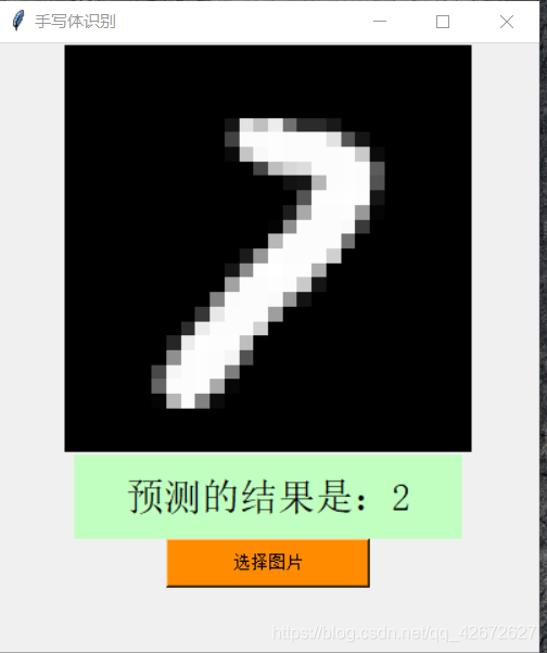
3.带界面的识别demo

import tensorflow as tf
import numpy as np
import tkinter as tk
from tkinter import filedialog
from PIL import Image, ImageTk
#import Image, ImageTk
from tkinter import filedialog
import time


def creat_windows():
    win = tk.Tk() # 创建窗口
    sw = win.winfo_screenwidth()
    sh = win.winfo_screenheight()
    ww, wh = 400, 450
    x, y = (sw-ww)/2, (sh-wh)/2
    win.geometry("%dx%d+%d+%d"%(ww, wh, x, y-40)) # 居中放置窗口

    win.title('手写体识别') # 窗口命名

    bg1_open = Image.open("timg.jpg").resize((300, 300))
    bg1 = ImageTk.PhotoImage(bg1_open)
    canvas = tk.Label(win, image=bg1)
    canvas.pack()


    var = tk.StringVar() # 创建变量文字
    var.set('')
    tk.Label(win, textvariable=var, bg='#C1FFC1', font=('宋体', 21), width=20, height=2).pack()

    tk.Button(win, text='选择图片', width=20, height=2, bg='#FF8C00', command=lambda:main(var, canvas), font=('圆体', 10)).pack()
    
    win.mainloop()

def main(var, canvas):
    file_path = filedialog.askopenfilename()
    bg1_open = Image.open(file_path).resize((28, 28))
    pic = np.array(bg1_open).reshape(784,)
    bg1_resize = bg1_open.resize((300, 300))
    bg1 = ImageTk.PhotoImage(bg1_resize)
    canvas.configure(image=bg1)
    canvas.image = bg1

    init = tf.global_variables_initializer()

    with tf.Session() as sess:
            sess.run(init)
            saver = tf.train.import_meta_graph('save/model.meta')  # 载入模型结构
            saver.restore(sess, 'save/model')  # 载入模型参数
            graph = tf.get_default_graph()       # 加载计算图
            x = graph.get_tensor_by_name("x-input:0")  # 从模型中读取占位符变量
            keep_prob = graph.get_tensor_by_name("keep_prob:0")
            y_conv = graph.get_tensor_by_name("y-pred:0")  # 关键的一句  从模型中读取占位符变量
            prediction = tf.argmax(y_conv, 1)
            predint = prediction.eval(feed_dict={x: [pic], keep_prob: 1.0}, session=sess)  # feed_dict输入数据给placeholder占位符
            answer = str(predint[0])
    var.set("预测的结果是：" + answer)

if __name__ == "__main__":
    creat_windows()
1
2
3
4
5
6
7
8
9
10
11
12
13
14
15
16
17
18
19
20
21
22
23
24
25
26
27
28
29
30
31
32
33
34
35
36
37
38
39
40
41
42
43
44
45
46
47
48
49
50
51
52
53
54
55
56
57
58
59
60

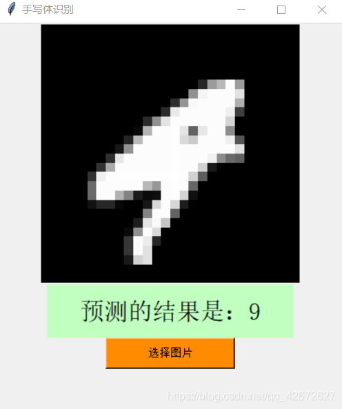
运行结果

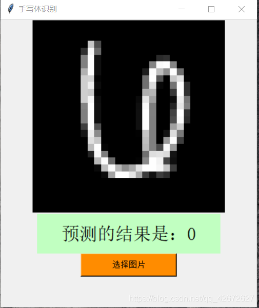
正确匹配：

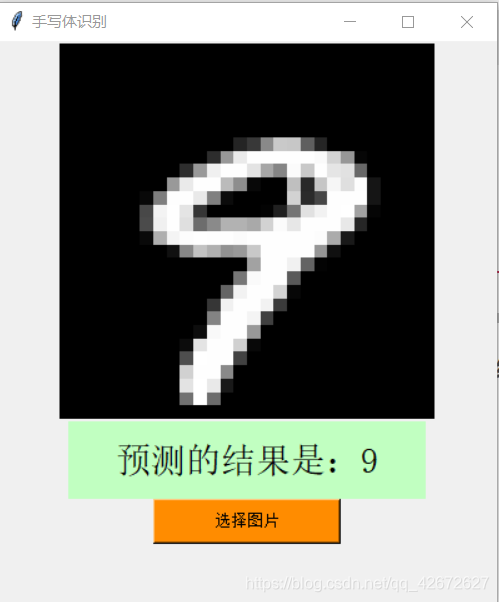
只要图像偏差不是很大，预测的准确率还是可观的。

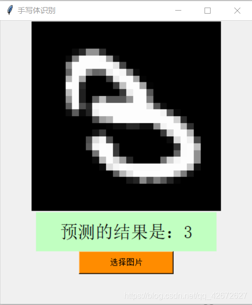
错误匹配：

把1预测成8的情况：图片整体怎么看也不像8，预测错误。

把1预测成6，这边的1确实有点偏差，导致预测出差。

把4预测成9，这边图片确实模棱两可，像4又像9，图片问题。

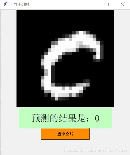
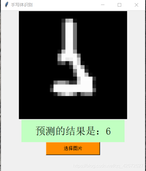
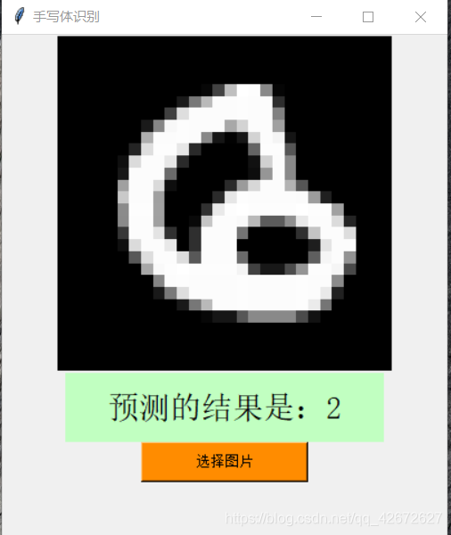
这边把6预测成2和0，数字不太整齐，可能环形的字体让预测出现偏差。

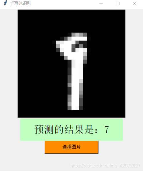
下面分别把9预测成7,7预测成2。图片上没多大问题，字体也整齐，这边可能是模型估测的偏差。

错配总结

（1） 一些字体在书写上的不规范，奇形怪状导致模型预测出现错误。
（2） 有些数字，比如3，6，8，9比较相似，在预测时容易形成错配，特别是7/4，9/4这两组数字，错配率明显。
（3） 模型上的不成熟，导致一些简单的图片也有可能出现错配，当然正确率百分百的模型并不存在，这样模型的准确率算是很高了。
（4） dropout 在防止过拟合时，屏蔽掉了一些正确输出（当然只是少量），导致损失函数判定分类时出现偏差。

这边只是个人分析总结，当然可能还有一些点没提到的 望补充。